Lecture 8: Assembly - Towards a Long Reads Assembler

Lecture 8: Assembly - Towards a Long Reads Assembler

Thursday 1 February 2018

Topics

1. Errors
   • Impact of errors on greedy algorithm
   • Impact of errors on k-mer algorithms
   • Prefiltering to Remove Error Reads
   • Read-overlap graphs
2. Partial Reconstruction
3. Introduction to Alignment
   • Types of errors
   • Edit Distance

Errors

Our discussion in earlier lectures assume perfect reads with no errors; however, this is not the case in practice. There are always errors present during sequencing and base-calling. We want to therefore answer the question: What is the impact of errors on assembly? How do we account for these errors in the algorithms we have presented?

Impact of errors on greedy algorithm

Lets first consider the greedy algorithm and how errors will impact its performance. Recall that this algorithm merges the two reads with the longest overlap.

If there are errors present, we won’t be able to find a perfect overlap and the longest overlap may be corrupted by errors (and would be considered not an overlap by the algorithm).

To account for the errors, not only do we account for perfect overlap, but we must also consider approximate overlap. For example, an approximate overlap of 99% would mean that 99% of the overlapped nucleotides match while the other 1% do not. This percentage depends on the error rate. The approximate percentage should intuitively be = (1 - 2 x error rate). For example, a 1% error rate may cause 1% error on each side of the overlapped reads, thus there would be a possibility of a 2% error. The approximate percentage overlap would then be 98%.

Impact of errors on k-mer algorithms

Now lets consider the class of k-mer algorithms. We will use an example to show how an error may affect our k-mer graph.

Consider a sequence of letters (we will use the English alphabet instead of A,G,C,T in this case) and the three reads of length 5:

Here, L = 5 and k = 3. The k-mers from the 3 reads are:

We can therefore create a k-mer graph from this 3 reads as follow:

Now suppose we have a third read, OWORL. But this read is corrupted and has an error, so we read OWXRL instead. The k-mers for this read are OWX, WXR, XRL. Therefore, combining this third read we have:

The error read creates a new path in the k-mer graph that branches out and may then be connected back to the main path. This branched out path is called a bubble.

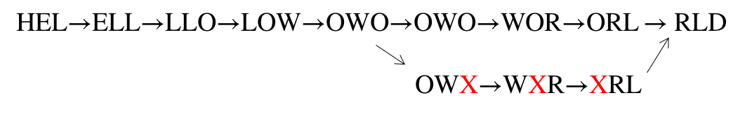
The error read creates a new path in the k-mer graph that branches out and may then be connected back to the main path. This branched out path is called a bubble. In practice, our dataset is large and we have a large number of reads. We may have both OWORL and OWXRL reads in our dataset. With bubbles, we will have two possible paths. This would create ambiguity in finding the Eulerian path from the k-mer graph.

There are methods used to address these:

1. We can align the two possible paths and choose the path that occurs more often. Since the error path is rare, there is a higher probability that the correct path will occur more often. Thus, choosing the more common path would eliminate the error bubble.
2. We can filter out reads that contain errors before actually creating our k-mer graph.

Prefiltering to Remove Error Reads

To find reads that contain errors in our dataset, we must consider the probability of correct reads occurring in our dataset as well as the probability of incorrect reads (errors) occurring.

So how many times will a particular k-mer appear, assuming that there are no error?

If we have k = 20, L = 100, and coverage = 30,

If we have an error rate of 1%,

Therefore,

Thus, a k-mer of length 20 will occur 20 times on average with no errors out of the 24 times that it may appear. Now consider the case with 1 error:

Therefore

Approximately 1 out of the 24 k-mer that occurs will have an error. We can therefore easily find the k-mer that rarely appears or in few numbers and discard them as error reads. We can set a threshold on the number of occurrences of a particular k-mer for it to be a valid k-mer.

Now lets consider a higher error rate of 15%, the error rate associated with long-read sequencing. Doing the same calculation we have that:

A k-mer with no errors will appear rarely as well in this case. This means that it is very hard to tell if a k-mer that appears once is an error k-mer or a valid one. We won’t be able to set a threshold and pre-filtering breaks down at large error rates. We can prevent breakdowns by setting smaller k values (using smaller k-mers), but this approach may not be practical because of the huge size of our resulting k-mer dataset. Therefore with higher error rate, people usually do not use k-mer based algorithms and instead will choose to use read-overlap graph algorithms which do not have this problem.

Read-overlap graphs

Taking a step back, we realize that the process of chopping longer reads into short k-mers seems like a strange paradigm since the reads contain all the information to begin with (why chop them up only to bring them back?). A more natural class of algorithms are based on read-overlap graphs, which is actually the original approach to assembly.

Instead of thinking about k-mers, we should think about reads themselves. Using this idea, we reconstruct a graph where all the nodes of the graph are reads (without any k-mer transformation). Then, we connect every pair of nodes with an edge, building a complete graph. Each edge is associated with a number that indicates the amount of overlap between the two nodes (reads). Alternatively, we can also associate each edge with a number that indicates how much length we gain by joining the two reads.

An example of a read-length graph is shown below. If you have two reads ACGCA and CGCAT, you would get an extension of 1 (overlap of 4) when the reads are put together to form ACGCAT.

A read overlap graph contains the original sequence as a Hamiltonian path.

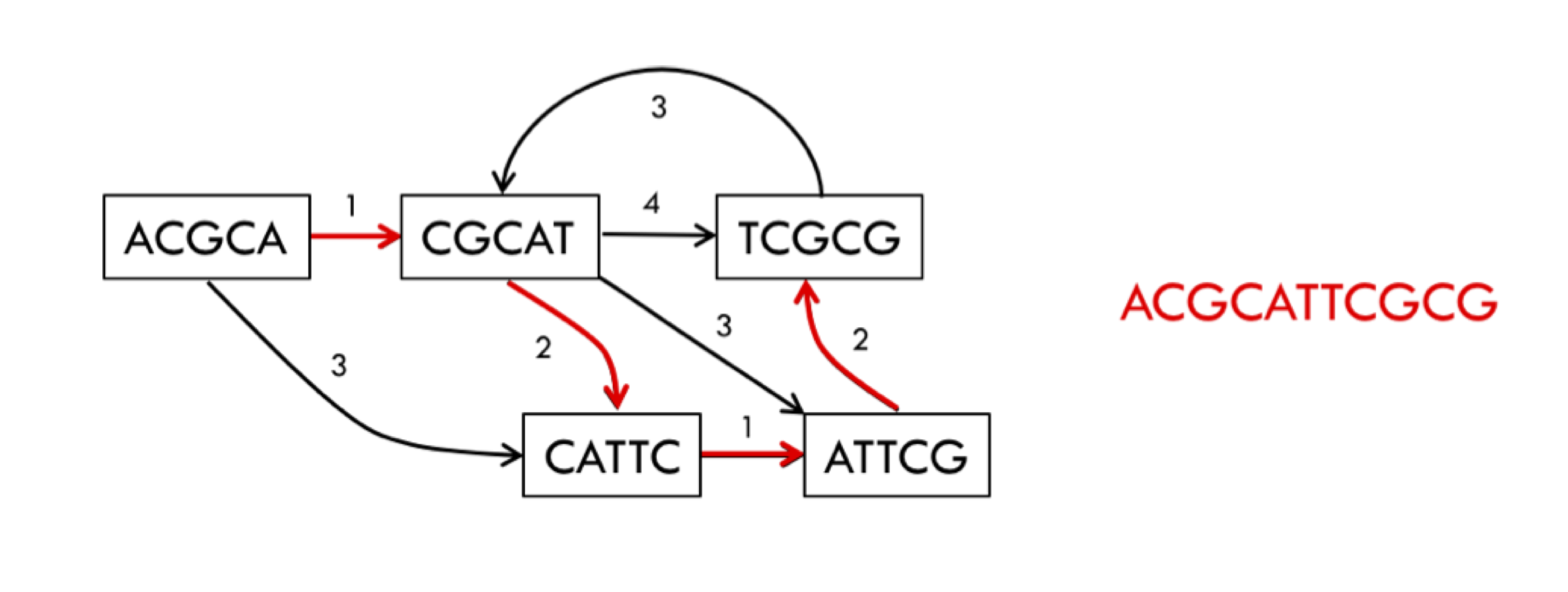
In some sense, this is the most natural representation of the assembly problem. To solve the problem we would take a path that goes through every single node in the graph while also minimizing the sum of the extensions (or maximizing the sum of the overlaps). This path is called the Generalized Hamiltonian Path, a path that visits every node at least once while maintaining the minimum sum of weights (note the difference between this and the Eulerian path). We may need to visit a node multiple times due to repeats. It turns out that this problem is NP-hard. This is one of the main motivations for working with the de Bruijn graph instead.

Partial Reconstruction

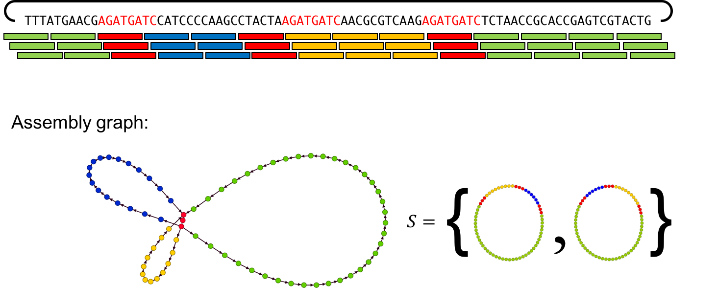
As previously discussed, there are regions of the genome that people cannot assemble because the repeats are so long. Especially for complex genomes, it’s difficult to perfectly reconstruct the genome. Instead, we introduce the concept of a partial reconstruction, or some way to convey the areas of ambiguity in the genome along with the areas we can reconstruct with high confidence. We can convey all the information we have using an assembly graph.

An assembly graph corresponding to a genome that's impossible to perfectly assemble. There are multiple (2) Eulerian paths, and each corresponds to a legitimate assembly. This can be viewed as assembling upto log (2) = 1 bit of uncertainty.

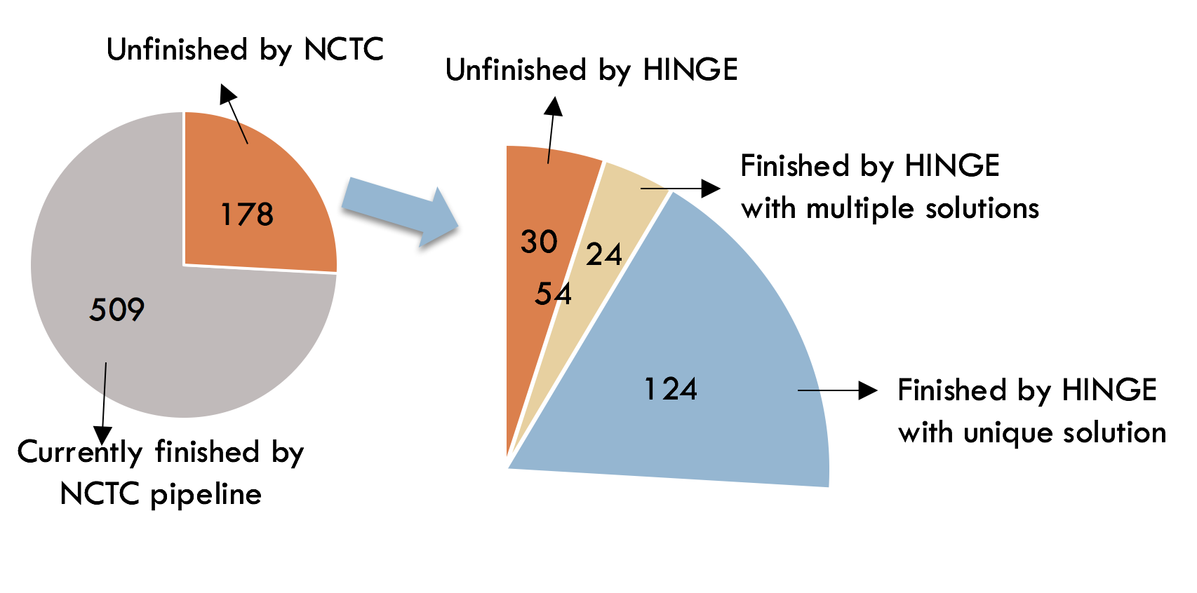
Older long read assemblers include HGAP, PacBio’s long-read assembler, and Miniasm and have trouble assembling genomes with these repeat-based ambiguities. A novel long-read assembler called HINGE attempts to fix this problem by generating assembly graphs and then resolving resolvable repeats on them. This seems to be a viable algorithm and seemed to improve assembly on the unfinished data sets of the Public Health England bacterial reference collections assembling many of them to completion and giving a graph solution to many others.

HINGE finishing a good fraction of unfinished assemblies of the Public Health England bacterial reference collections dataset. Finished by HINGE with multiple solutions means that an assembly graph with multiple Eulerian cycles is obtained.

Introduction to Alignment

We have talked about assembling the genome from reads; however, before assembly we need to first merge two reads by aligning them with parts that overlap. We will now discuss how we solve this alignment problem. Because of errors, we will consider an algorithm that does an approximate alignment to find overlapping reads. There are two important problems where alignment is useful:

1. Finding overlapping reads for a de novo assembly.
2. Comparing reads with a reference genome to see which region the read belongs to. In turn we can find new variations and differences in the reads from the reference genome.

Type of Errors

Using the example sequence AGGCTTAAT, we describe three types of errors:

1. Substitution: AGGCCTTAAT
2. Insertion: AGGCTTAAAT
3. Deletion: AGGCTT-AT

Second generation technologies like Illumina have mainly substitution errors at a rate of around 1-2% Third and fourth generation technologies like PacBio and Nanopore have no PCR, and hence the error rate is \(\approx\) 10-15% with mainly insertion and deletion errors.

Edit Distance

To solve the alignment problem, we want to find the best way to align two strings by taking into account the three different types of errors we discussed earlier. Consider two strings \(x\) and \(y\):

x = GCGTATGTGGCTAACGC
y = GCTATGCGGCTATACGC

In order to measure how much these two strings overlap, we will consider the edit distance of the two strings. Edit distance is defined as the the minimum # of insertions, deletions and substitutions necessary to get from string x to string y. Using the x and y given, we will denote a deletion by a -, and a substitution by a red letter.

x = GCGTATGTGGCTA-ACGC
y = GC-TATGCGGCTATACGC

We see from our example that we have two insertion/deletions at the 3rd and 14th letters of the sequence and a substitution at the 8th letter. Therefore there are 3 edits, resulting in an edit distance of 3.

One could compute edit distance between two strings by computing all combinations of insertions, deletions, and substitutions on the first string until we arrive at the second string. This brute-force approach will take exponential time in terms of the length of the string and is not efficient. An efficient solution would be to use Dynamic Programming.

An algorithm to find the edit distance would require us to break down the problem into subproblems. Using solutions from the subproblems, we can then build a working solution for the whole problem. We will discuss this algorithm next lecture.