Lecture 5: Assembly - An Introduction
Lecture 5: Assembly - An Introduction
Tuesday 23 January 2018
Topics
ISI and deletion
We ended last lecture with a discussion on base calling for Oxford Nanopore’s technology, summarized by the following figure:
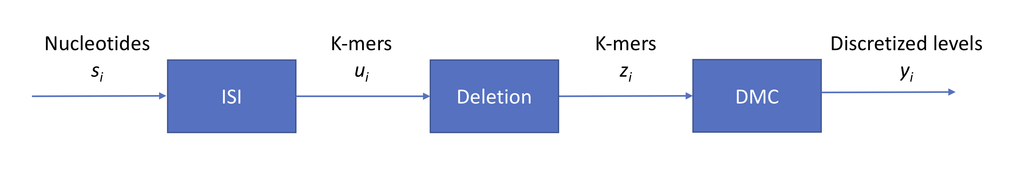
We have three sources of noise:
- context (intersymbol interference): each signal read from the nanopore is an aggregate from individual signals from multiple symbols
- indels (insertions and deletions): the strand does not pass through the pore at a constant speed
- technical: measurement noise which we model as additive Gaussian zero-mean noise
Last time, we also discussed how we can decode a series of length-4 contexts (sliding 4-mer windows) using a trellis and the Viterbi algorithm. A point of confusion stemmed from how the algorithm would perform in the event of an indel. We will discuss the deletion event in more detail. Without a deletion, each initial context can transition to one of four states (e.g. AAAA, AAAC, AAAG, AAAT for the initial context AAAA). Each intermediate trellis stage contains \(4^4 = 2^8\) states, and each node at stage \(i\) will have 4 outgoing edges connecting the node to stage \(i+1\). For a deletion event, we can add edges to states AATA, AATC, etc. to account for other 4-mer contexts that AAAA can transition to. In other words, we simply need to add more edges to the trellis. Running Viterbi now will result in a sequence that’s 1 longer than the number of intervals estimated from the analog signal.
Perhaps counterintuitively, the ISI due to the context can be useful (see Question II part 5 on assignment 1). If we miss a base, we have 3 contexts that contain information about the base.
Review
So far in the course, we have discussed three different technologies in detail: second-generation sequencing (Illumina), Oxford Nanopore, and PacBio.
| Second gen. (Illumina) | Oxford Nanopore (MinIon) | PacBio | |
|---|---|---|---|
| read length (bases) | 100-500 | 10K-100K | 10K-20K |
| error rates | < 1% | 10-15% | 10-15% |
| speed (time/base) | 6 mins/base/strand | 250 bases/s | 3 bases/s |
| # of reads in parallel | \(10^9\) | 2000 | 150K |
| throughput (total # of bases/s) | 3M | 500K | 450K |
Reads from a sequencer
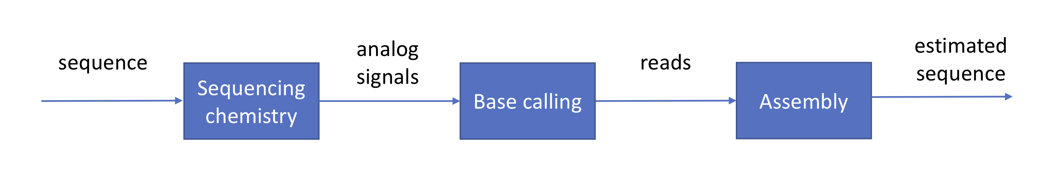
We have already gone through a high-level description of the roles of the sequencer and the base caller and how these are achieved in practice. Assuming that these stages are completed successfully, their output would be hundreds of millions to billions of erroneous reads. This information is usually provided to us in the format of a FASTQ file in which \(Q\) stands for the quality score associated to each base:
\(P_e\) is the probability of error calculated in the base calling stage. The next phase in the pipeline is to reconstruct the original sequence from read data.
The genome assembly problem
The genome assembly problem is the following: Given reads coming from a sequence, how does one reconstruct the sequence? There are two relevant flavors of this problem.
- reference-based assembly: reconstructing the genome while leveraging side information from a reference, such as an already-assembled genome. This is useful for SNP calling, or the process of determining which individual bases of an organism’s genome is different from the reference
- de novo assembly: reconstructing the genome from just the reads. This is relevant in cancer and when a previously unsequenced organism is sequenced for the first time
We will focus mainly on de novo assembly, and we will attempt to answer the following questions:
- How many reads do we need to assemble?
- How do we design efficient assembly algorithms that can operate with the minimum number of reads and read length?
Coverage
Starting with some notation, let
\[\begin{align*} G &= \text{Length of the genome},\\ L &= \text{Read length},\\ N &= \text{Number of reads}. \end{align*}\]We assume that \(L\) is fixed. We first derive a relationship between the above three values that would result in successful assembly. Since \(L\) and \(G\) are fixed with our choice of experiment and technology, we need to choose \(N\) (i.e. “How much sequencing do I need to do?”). Intuitively, the reads must cover the entire genome, and each base has to be covered by at least 1 read. Therefore \(LN > G\) or \(N > G/L\). In order to achieve this lower bound, we need to have all \(LN\) reads aligning perfectly without overlap, which is highly unlikely.
It turns out that if we let \(\epsilon\) represent the probability of not achieving full genome coverage, then
\[N \geq \frac{G}{L} \ln \frac{G}{\epsilon}.\]If this condition is met, then we have achieved coverage with probability \(\geq 1-\epsilon\). This result is more stringent than our previous bound due to the \(\ln (G/\epsilon)\) term, which is greater than 1.
In isolation, \(N\) is not too informative. For a particular sequencing experiment, \(N =\) 100 million reads could be large or small depending on the size of the genome and the length of each read. Because the reads are random, some bases will be covered more often than other bases. Therefore rather than using \(N\), we are instead interested in the coverage depth, or the average coverage per base, which is described by
\[c = \frac{NL}{G} \geq \ln \frac{G}{\epsilon}.\]As an example, if the genome of interest is about one billion base pairs long, then we need at least \(25\)x coverage depth since \(G=10^9;\epsilon=0.01\Rightarrow c=25.328\ \\). The number of reads covering a position is exactly binomial with parameters \(\left(N, \frac{L}{G}\right)\). Note that \(\frac{L}{G}\) is quite small, and therefore the number of reads can be approximated with a Poisson distribution with mean \(c= \frac{NL}{G} \\).
As a parting thought, we observe that this condition holds for every \(L\). Suppose \(L = 1\) (each read is only 1 base long). The condition in its current form states that we can assemble if we have a large enough \(N\), but intuitively this is wrong. We will address this next lecture.