Lecture 3: Base Calling for Second-Generation Sequencing

Lecture 3: Base Calling for Second-Generation Sequencing

Tuesday 16 January 2018

Topics

In the previous lecture, we learned about the evolution of first and second generation sequencing efforts. In this lecture, we examine the base calling step: the inference of individual bases from a series of light intensity signals.

1. Introduction
2. Error sources
   • The error model
   • Inference on the model
     • Zero-forcing
     • Minimum mean square error based estimation
     • Maximum likelihood estimation

Introduction

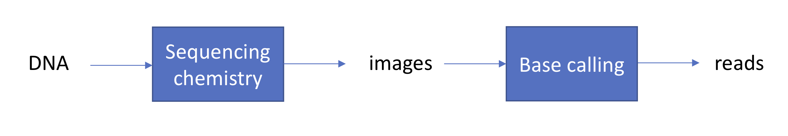
We begin with a review of the sequencing by synthesis approach to sequencing. We start with DNA and fragment it into many shorter sequences (resulting in a number of fragments on the order of 100 million to 1 billion). We then hybridize (or “stick”) the fragments onto a glass slide called a flow cell. We recall that sequencing by synthesis begins with ddNTP (free-flowing) and DNA polymerase, which binds both dNTP and ddNTP. In addition, we introduce an enzyme that reverses termination in each washing cycle. We also introduce some chemistry to capture florescence signals each time a ddNTP binds, and we record these signals by taking pictures (one picture per nucleotide per cycle, for example).

The process of obtaining reads from DNA.

We note that the above is a simplified version of base calling. In reality, the fluorescent signal from a single template is too weak to be detected. Hence, first the template is converted into many clones using a technique called polymerase chain reaction (PCR) (which also won its discoverer Kary Mullis a Nobel prize). Before synthesis, each strand is cloned using PCR and each dot becomes a clonal cluster corresponding to 1000s of clones per strand.

Ideally one would want all copies of fragments in a cluster to be synchronized in their synthesis process going forward. Because of chemical and mechanical imperfections, some strands are lagging behind and others are leading forward in the same cluster. This puts up challenges for doing inference which are handled with some clever signal processing.

Error sources for Illumina sequencing

The main source of errors is the asynchronicity of the various molecules in a dot stemming from the randomness intrinsic to chemical processes.

During the washing away of the dNTPs step, a small fraction of dNTPs will inevitably remain. Therefore for some DNA molecules, DNA polymerase will attach a dNTP rather than just a ddNTP. The synthesis will not be terminated, and the polymerase will ultimately attach both a dNTP and a ddNTP. This results in some strands being one or more bases longer than normal. These strands are said to be leading.

Because enzymes are not perfect, another error would occur if termination is not reversed in the washing cycle. Therefore some strands will miss a cycle and be one base shorter than normal. These strands are said to be lagging.

A visual comparison of normal, leading, and lagging events in second-generation sequencing.

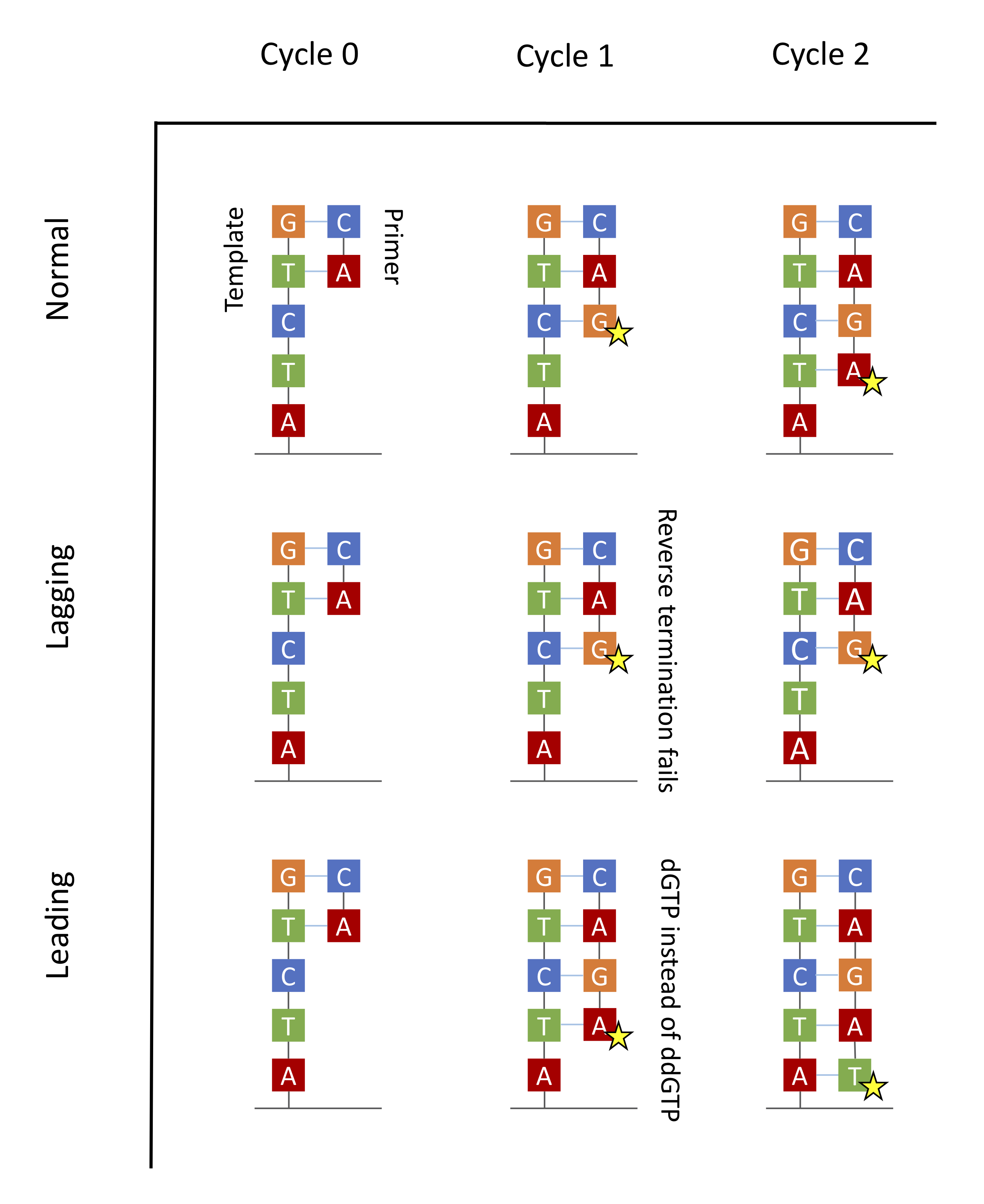
Both leading and lagging errors are called phasing errors.

The error model

We probabilistically model the problem as follows. Let \(L\) be the length of the molecule being sequenced. Let the original sequence be \(\mathbf{s}=s(1),s(2),\cdots,s(L).\) Let us define sequences \(\mathbf{s}^{(A)},\mathbf{s}^{(C)}, \mathbf{s}^{(G)}, \mathbf{s}^{(T)}\) as

Let \(\mathbf{y}^{(A)}, \mathbf{y}^{(C)}, \mathbf{y}^{(G)}, \mathbf{y}^{(T)}\) be the intensities of the colours corresponding to A, C, G, and T respectively. We note that we make \(L\) measurements in total (one measurement per cycle), and hence each one of \(\mathbf{y}^{(A)}, \mathbf{y}^{(C)}, \mathbf{y}^{(G)}, \mathbf{y}^{(T)}\) is an \(L\) length vector.

A naive way of converting the intensities to bases is by simply looking at which base corresponds to the maximum intensity signal. We can do better by exploiting the fact that the system has memory and looking at images from different cycles jointly rather than independently. If a strand lags or leads for a cycle, then the entire sequence is shifted by one base.

A key step in signal processing is building a model for how noise is added to the signal. Specifically, we want to capture how the original clean signal \(\mathbf{s}^{(A)}\) becomes distorted due to two sources of noise:

1. The signal observed in cycle \(j\) depends not only on \(s^{(A)}(j)\) but upon all other values of \(\mathbf{s}^{(A)}\). In statistical signal processing, this is called inter-symbol interference (ISI).
2. Technical noise added by the sequencing process.

Since we have a lot of copies per clonal cluster, we can assume that the channel, which models how the signal becomes distorted, is deterministic and can be described by some average distortion on the input signal (law of large numbers). We will assume that the technical noise is additive, resulting in the following model diagram:

Modeling the base calling process.

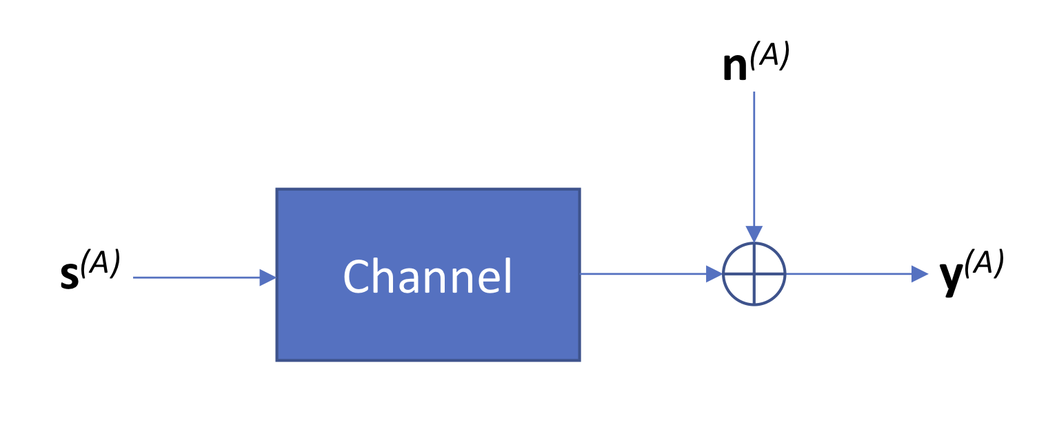
We define

Note that we are assuming that the probability of binding more than one dNTP in a cycle is negligible, and therefore we omit it from the model. Further we define

For example, if \(p = q = 0\), then \(Q\) would just be the identity matrix. In general, \(Q_{11} = 1-p-q, Q_{21} = (1-p-q)p, Q_{31} = (1-p-q)p^2, \dots \ \ \\) As we move farther away from the diagonal entries of the matrix, the probabilities get smaller. Now we model the relationship between \(\mathbf{y}^{(A)}\) and \(\mathbf{s}^{(A)}\). Here we observe that at time \(i\), the intensity is given by

where \(n_i\) is noise that we model as zero mean Gaussians \(\mathcal{N}(0,\sigma^2)\), independent across cycles, and \(b\) is the total intensity expected if all molecules had the same colour emitted.

In matrix notation, this problem reduces to

Inference on the model

Zero-forcing

The most obvious inference rule would be

where \(\mathbb{I}\) is the usual indicator function, that is

In signal processing literature, this is referred to as Zero-forcing, a brute-force method that cancels out the ISI.

We note that

where \(\mathbf{n}_{ZF} \sim \mathcal{N}(0, \sigma^2 Q^{-1}(Q^{-1})^{T})\) . That is, the noise across coordinates are not independent. This means we are losing information using the Zero-forcing strategy since we are not exploiting the fact that the noise changes over time.

Additionally, this formulation is suboptimal if \(Q\) is an ill-conditioned matrix, i.e. if the largest singular value of Q is much larger than the smallest singular value of Q. To see this at a high level, let \(\sigma_{\max}^2, \sigma_{\min}^2\) be the largest and the smallest singular values of \(Q\). Next note that the noise variance of \(n_{ZF}\) in the dimension corresponding to the largest singular value of \(Q\) is \(\frac{\sigma^2}{\sigma_{\max}^2}\), which is much smaller than \(\frac{\sigma^2}{\sigma_{\min}^2}\), the noise variance of \(n_{ZF}\) in the dimension corresponding to the smallest singular value of \(Q\). The probability of making an error is determined to a first order by the latter which can be quite bad.

Minimum mean square error based estimation

Another popular estimator is the Minimum mean square error (MMSE) estimator.

Here we first approximate \(\mathbf{s}^{(A)}\\) to be distributed according to \(\mathcal{N}\left(\frac{1}{4} \mathbf{1}, \frac{3}{16} I \right)\) . This approximation is reasonable as every co-ordinate of \(\mathbf{s}^{(A)}\\) can be modeled as Bernoulli\(\left(\frac{1}{4}\right) \\), and the Gaussian approximation is by matching the first and second moments of the Bernoulli.

Then we find the \(\hat{\mathbf{s}^{(A)}}\) such that \(\mathbb{E}[(\hat{\mathbf{s}^{(A)}}-\mathbf{s}^{(A)})^2]\) is minimized. In the standard setting when the support of \(\mathbf{s}^{(A)}\) is not restricted to be \(\{0,1\}\), this leads to \(\hat{\mathbf{s}^{(A)}}= \frac{3}{16} bQ^T\left( \frac{3}{16} b^2 QQ^T+\sigma^2 I\right)^{-1}\left(\mathbf{y}^{(A)} - \frac{1}{4}b Q \mathbf{1}\right) + \frac{1}{4}\mathbf{1}\ \\).

Hence the MMSE-based estimator used in this setting is

One drawback of this method is that it does not use the fact that \(\mathbf{s} \in \{0,1\}^{L}\) and the fact that for any co-ordinate \(i\) exactly one of \(\mathbf{s}^{(A)}(i), \ \mathbf{s}^{(C)}(i), \ \mathbf{s}^{(G)}(i), \ \mathbf{s}^{(T)}(i)\ \\) is equal to \(1\).

Maximum likelihood estimation

The maximum-likelihood estimator for this case would involve running the Viterbi algorithm. This basically involves solving

Unlike for the MMSE method, we no longer have a prior on \(\mathbf{s}\). Instead, we simply want to choose the \(\mathbf{s}\) that maximizes the likelihood of what we observe. The time complexity of the Viterbi algorithm is exponential in the recursion depth (which in here is the maximum |i-j| if there is non-zero probability of seeing light from base j at time i). In this setting, this is \(O(2^{L})\). A work-around this is to approximate each column of \(Q\) so that it is non-zero only in a \(w\) width band. This gives the run time of the maximum-likelihood to be \(O(2^{w}L)\). This is quite managable for \(w \le 10\).