Lecture 19: Single-Cell RNA-Seq - Clustering
Lecture 19: Single-Cell RNA-Seq - Clustering
Tuesday 13 March 2018
scribed by Daniel Hsu and edited by the course staff
Topics
Introduction
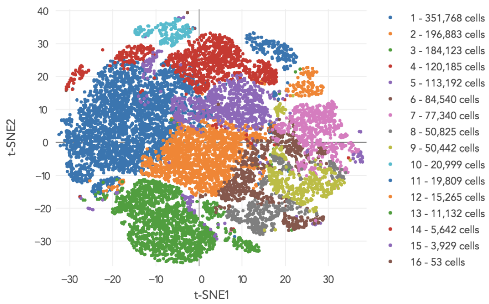
The clustering problem can be posed as follows: we start with several data points of dimension \(p\). For the single-cell dataset mentioned last lecture, we had \(n = 1,300,000\) cells and \(p = 2000\) after some preprocessing. The goal of clustering is to partition the \(n\) cells based on some notion of distance.
K-means
For \(K\)-means clustering, distance is defined as
\[\text{dist}(y_1, y_2) = \|y_1-y_2 \|_2^2.\]We define our set of observed points as \(G = \{y_1, y_2, \dots, y_n \}, y_i \in \mathbb{R}^p \ \\). We assume that the true number of clusters is \(K\), and therefore we want to partition \(G\) into \(K\) subsets such that \(G = G_1 \cup G_2 \cup \dots \cup G_K\). We note that practically, \(K\) may not be known a priori and therefore one may need to test several \(K\)’s. For now, we will assume \(K\) is known. The \(K\)-means formulation is as follows:
\[G_j \rightarrow r_j \in \mathbb{R}^p \text{ (representative or center of } G_j \text{)}.\]In other words, we associate each cluster with some representative. We then cluster by assigning \(y_i \rightarrow z_i \in \{1, 2, \dots, k\}\\), \(z_i\) being the label of cluster containing point \(i\). Thus the representative point there is \(r_{z_i}\).
The \(K\)-means optimization problem can be formally stated as:
\[J = \min_{\{z_i\}, \{r_j\}} \sum_{i=1}^n \|y_i - r_{z_i}\|^2.\]This objective captures how we want to pick the centers \(r_j\) and cluster assignments \(z_i\) such that the distances from points to assigned cluster centers are small. It turns out that this problem is somewhat difficult to solve. For one, it’s non-convex. This problem is typically solved using an iterative approach. Note that we have two sets of variables we are optimizing over (\(z_i\)s and \(r_j\)s). Therefore we can fix one set of variables and see if we can optimize the other set.
Optimizing assignments: Given \(\{r_j\}\) (i.e. centers are fixed), how do we find \(\{z_i\}\)? For every \(i\), we can solve the optimization problem
\[\min_j \| y_i - r_j \|^2.\]We assign each point \(y_i\) to the closest center.
Optimizing centers: Now, if we are instead given \(\{z_i\}\) (i.e. assignments are fixed), can we optimize over \(r_j\)? Note that the only points that contribute to a cluster center \(r_j\) are those points assigned to cluster \(j\) (i.e. points that end up in \(G_j\)). Again we can break up the optimization problem into isolated optimizations (one for each cluster \(j\)):
\[\min_r \sum_{i \in G_j} \|y_i - r \|^2.\]The solution to this problem is the center of mass (i.e. the value that minimizes the sum of moments of inertia given that each \(y_i\) is some point mass in a physical system)
\[r_j^* = \frac{1}{|G_j|} \sum_{i \in G_j} y_i.\]We now have a chicken and egg problem. The \(K\)-means algorithm proceeds as follows:
\[\{ z_j^{(0)}\} \rightarrow \{r_j^{(0)}\} \rightarrow \{z_j^{(1)}\} \rightarrow \{r_i^{(1)} \} \rightarrow \dots\]That is it starts from a random assignments of points to clusters and then finds the best representative points for this labelling of the points. Then it uses the labelling to improve the clusters, and then recompute the labelling. It continues in this manner.
We are interested in two questions:
- Will this algorithm even converge?
- Will this algorithm work for large amounts of data, like the \(n\) and \(p\) given for the 10x dataset?
Note that for each mini-optimization, we reduce the value of our overall objective function. Because the objective is non-negative (as it’s the sum of squared terms), and because each optimization can only decrease the value of the objective, \(K\)-means is guaranteed to converge. Unfortunately, it may not necessarily converge to a global optimum. In practice, users tend to test a few different initializations and simply pick the best result. Other approaches such as \(K\)-means++ intelligently chooses initial centers.
Intuitively, the computational cost must depend on the number of points \(n\) and the dimension \(d\).
- Finding the nearest neighbor for every point requires \(O(nKd)\) operations, since that point needs to be compared to each of the \(K\) representative points.
- Finding the center of mass also requires \(O(nd)\) operations, since each point is only used once in the computation of one of the centers
Therefore each iteration is linear in \(n\). In practice, the number of iterations required for convergence is typically not too large.
Importantly, if the distance measure changes (for example, perhaps we are interested in
\[\text{dist}(y_1, y_2) = |y_1-y_2 |\]the \(L_1\) distance, instead of the \(L_2\) distance given above), then the nearest neighbor computation for each point remains \(O(Kd)\). The computation of the center of mass, however, becomes the computation of the co-ordinate wise medians of the points in a cluster. Thus it takes \(O(nd)\) operations as well. However for other distances, this might not be the case.
EM on Gaussian mixture
This notion of iterative optimization might remind you of a previous algorithm we have discussed: expectation maximization (EM). Recall that EM is different, however, because EM attempts to solve an optimization problem formulated probabilistically. In contrast, \(K\)-means is just an optimization problem with no probabilistic interpretation. Therefore to use EM, we need to come up with some model describing how the data points are generated.
We can use a Gaussian mixture model. Let \(Z_i \in \{1, \dots, K\}\) represents the cluster assignment of the \(i\)th data point. We can say that
\[P(Z_i = j) = p_j.\]We assume that conditioned on \(Z_i = j\), \(Y_i\) is a circular Gaussian with mean \(\mu_j\): \(Y_i \mid Z_i = j \sim N(\mu_j, I) \ \\). In other words, we assume that all points coming from a cluster are generated from some Gaussian distribution with a mean \(\mu_j\) unique to that cluster. More explicitly,
\[f(y_i; \theta) = \sum_j p_j \frac{1}{(\sqrt{2\pi})^p} \exp \left\{ -\frac{1}{2} \|y_i-\mu_j\|^2 \right\}\]The density for all \(n\) points \(Y = \{Y_1, \cdots, Y_n\}\) is
\[f(Y; \theta) = \prod_{i=1}^n\sum_j p_j \frac{1}{(\sqrt{2\pi})^p} \exp \left\{ -\frac{1}{2} \|Y_i-\mu_j\|^2 \right\}\]The hidden variables are \(\theta = (\mu_1, \dots, \mu_k, p_1, \dots, p_k)\ \\). Taking a log of \(f\), we obtain the log likelihood
\[\begin{align*} \ell_{\theta}(Y) & = \log f(Y; \theta) \\ & = \log \prod_{i=1}^n\sum_j p_j \frac{1}{(\sqrt{2\pi})^p} \exp \left\{- \frac{1}{2} \|Y_i-\mu_j\|^2 \right\} \\ & = \sum_{i=1}^n \log\left( \sum_j p_j \frac{1}{(\sqrt{2\pi})^p} \exp \left\{- \frac{1}{2} \|Y_i-\mu_j\|^2 \right\} \right) \end{align*}\]Maximizing \(\ell\) would give us the maximum likelihood value for \(\theta\):
\[\theta_\text{ML} = \max_\theta \log f(Y; \theta).\]This problem is not convex, and therefore running EM will only give us a locally optimal solution. Running EM will involve the following steps:
E-step: Fix
\[\theta: P(Z | Y; \theta) = \prod_{i=1}^n p(Z_i | Y_i ; \theta)\]Thinking intuitively, given that we have observed a data point \(Y_i\), we should obtain some posterior distribution of the clusters it could have come from. For example, a point on the boundary between two clusters might be assigned approximately \(1/2\) probability for coming from either of those clusters. Unlike for the \(K\)-means approach, which makes “hard” assignments (points are assigned completely to a cluster), EM gives us “soft” assignments. Therefore we can compute the posterior using
\[P(Z_i = j | Y_i ; \theta) = \frac{p_j \exp(-\|Y_i-\mu_j\|^2)}{\sum_{\ell} p_{\ell} \exp(-\|Y_i-\mu_{\ell}\|^2)}.\]This is easy to compute.
M-step: Fix
\[P(Z|Y)\]and compute
\[\begin{align*} \max_\theta E_{Z|Y} [\log P(Y, Z; \theta)] & = \max_\theta E_{Z|Y} \left[ \sum_{i=1}^n \log \left( \frac{p_{Z_i}}{(\sqrt{2\pi})^p} \exp \left\{\frac{-1}{2} \|Y_i-\mu_{Z_i} \|^2 \right\} \right) \right] \\ & = \max_\theta E_{Z|Y} \left[ \sum_{i=1}^n \left(\log p_{Z_i} - \frac{1}{2} \|Y-\mu_{Z_i}\|^2 \right) - \log(\sqrt{2\pi}^p) \right]. \end{align*}\]Given probabilities for cluster assignments (“soft” assignments),
\[\begin{align*} p_j^* & \approx \text{ total fractional assignment to cluster }j\text{ summed over all data points} \\ \mu_j^* & = \text{weighted average of } Y_i \text{'s (weight proportional to probability } Y_{ij} \text{ is assigned to } j \text{)} \end{align*}\]In some sense, perhaps EM is like some soft version of \(K\)-means. The E-step is analogous to the \(K\)-means step of assigning points to clusters, except for EM the points are assigned probabilistically based on the current parameters \(\theta\). Once the soft assignments are obtained, the parameters can be re-estimated, which is somewhat analogous to recomputing the cluster centroids. Importantly, the \(p_j\)’s were not present for \(K\)-means.