Lecture 18: Empirical Bayes and Single-Cell RNA-Seq Analysis

Lecture 18: Empirical Bayes and Single-Cell RNA-Seq Analysis

Thursday 8 March 2018

scribed by Brijesh Patel and edited by the course staff

Topics

1. Empirical Bayes
   • Recap of false discovery rate
   • Replicates in differential analysis
2. Single-cell RNA-Seq analysis

Empirical Bayes

Recap of false discovery rate

We have \(m\) hypothesis testing problems where we test whether each transcript is differentially expressed or not in condition \(A\) vs condition \(B\). We obtain \(m\) \(p\)-values from \(m\) statistical tests (one for each transcript), and we want to know which transcripts are actually differentially expressed.

One approach for justifying the Benjamini-Hochberg (BH) procedure is by viewing the \(p\)-values as drawings of some random variable \(P\) from an underlying distribution \(F\). Recall that under the null hypothesis, the \(p\)-value is distributed \(U[0, 1]\). Under the alternate hypothesis, the \(p\)-value will come from the some non-uniform (but unknown) distribution. The BH procedure attempts to estimate an empirical distribution \(\hat{F}\) from the data.

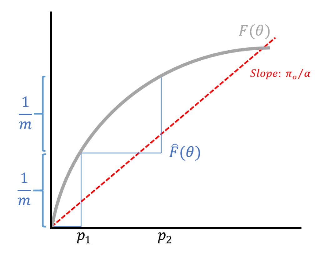
Once \(\hat{F}\) is computed, we can perform a transcript-by-transcript test where we evaluate if \(p_i \leq \theta\) for some decision threshold \(\theta\). From the discussion last lecture, we showed how \(\theta^*\) can be obtained using the expression

where \(\alpha\) is our lever of FDR control. If you know \(F\), then you can set your threshold to satisfy this equation. With our estimated \(\hat{F}\), we can rearrange the above expression to obtain

At any point \(\theta\), \(\hat{F}\) is (roughly speaking) the number of \(p_i\)’s which is less than \(\theta\):

Sorting the \(p_i\)’s, we obtain \(p_{(1)} < p_{(2)} < \dots < p_{(m)}\) where the inequalities are strict because the \(p\)-values are continuous. This results in a step-like function for \(\hat{F}\) as shown in the figure below.

Justifying the decision boundary for the BH procedure.

In conclusion, the BH procedure was a significant development in statistics it turns the multiple testing scenario from a nuisance to an advantage. Multiple testing can be viewed as an advantage of estimating, allowing us to estimate the distribution \(F\) so that instead of bounding a \(p\)-value, which is the probability we get a wrong discovery given that the null distribution is true, we can instead bound the probability we’ve made a mistake given that we’ve committed to a discovery. The latter is a more relevant metric, but requires modeling \(F\), which is a combination of the null and the alternate distributions. We cannot obtain an estimate of \(F\) without the data from the multiple testing problems. The BH procedure is a special case of the empirical Bayes theory.

Replicates in differential analysis

Recall that for differential expression analysis, we need more than one replicate in each condition. Otherwise, we would not be able to estimate variance or standard error (i.e. we would not be able to draw error bars). We obtain estimates for the mean and variances under the two different conditions A and B:

Here, \(X_i^A\) represents the expression level in the \(i\)th replicate under condition \(A\). Because getting replicates is expensive, we are interested in understanding the minimum number of replicates required such that we can draw reasonable conclusions. From a statistical testing point of view, our null hypothesis is that the two means and variances are equal:

Under the null, the variation stems from both technical and biological variation for both conditions. We use the mean and variance estimates above to compute a \(t\)-statistic:

The bigger the difference in means (i.e. the bigger the \(T\)-statistic), the more likely the null is invalid. In other words, whenever \(\hat{T}_n\) is large in magnitude, we are “suspicious of the null.” We start by comparing the \(t\)-distribution to the standard normal distribution \(N(0, 1)\):

Comparing the t-distribution with 2 degrees of freedom (red) to the standard normal distribution (blue).

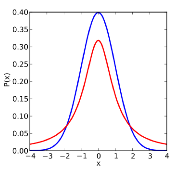
Note that the standard normal has smaller tails. This means that controlling the false positive rate for the \(t\)-distribution is more difficult, and we must use a larger cutoff in order to control the false positive rate, thus reducing the power of the test (to detect signal). If we knew the variance \(\sigma^2\), then the distribution of the \(T\) statistic would be Gaussian (a linear combination of Gaussians is Gaussian):

This highlights how significant the uncertainty in the variance estimate impacts the testing procedure; an underestimation of the variance results in a larger \(t\)-statistic. We can take a closer look at how the variance changes as a function of the data for \(n = 2\):

Variance estimate with respect to the data.

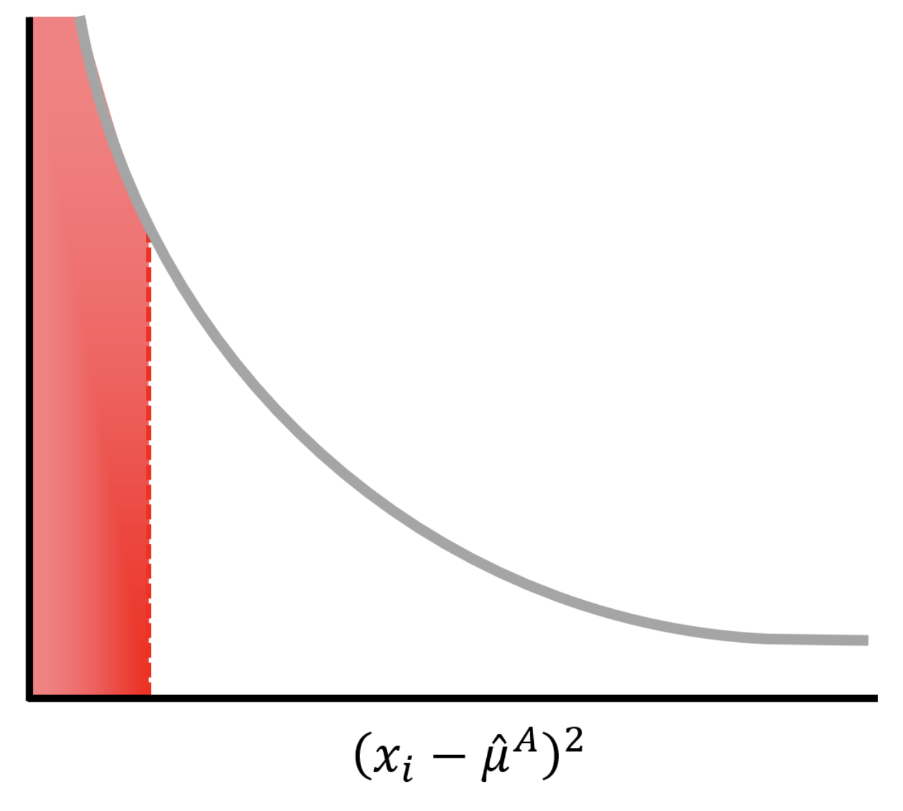
Because there is a large probability that \((x_i-\hat{\mu})^2\) is small (red area under the curve), our estimate of the variance and therefore the \(T\) statistic will be poor. As we increase the number of replicates, our performance gets better quickly.

Comparing the t-distribution with varying degrees of freedom (red) to the standard normal distribution (blue) as the number of replicates increases.

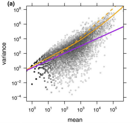
Empirical Bayes tells us that we can gain power by estimating some statistics associated all the data (i.e. by estimating some global prior using the data). DESeq leverages the information across genes to power a statistical test for differential expression. We can have a scatterplot of (sample mean, sample variance) for 20,000 genes. While the estimate for an individual gene may be poor, we can fit some (often parametric) model for all genes. This process is also known as shrinkage because we shrink the points towards our model, resulting in a tightening of the distribution. As shown in the figure, a Poisson model (blue) underestimates the variance in real data while a negative binomial distribution (orange) tends to fit the data better.

Modeling the expression across all genes in an RNA-Seq experiment using a Poisson model (purple) and a negative binomial model (orange). DESeq uses the latter model.

Single-cell RNA-Seq analysis

For the last part of the course, we will discuss various computational problems that arise from single-cell RNA-Seq analysis. A recent dataset published by 10x genomics consists of 1.3 millions cells and 28000 genes. Each cell is represented by a 28000-dimensional expression vectors.

The 10x Genomics 1.3 million cell dataset visualized in 2 dimensions using t-stochastic neighbor embedding.

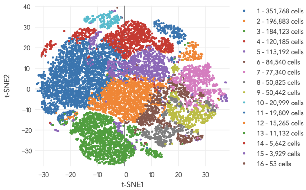
A typical pipeline would generate the above image as an output. After sequencing all these cells, we would like gain a sense of how many cell types there are. In contrast, bulk RNA-Seq gives us an average of all the cells in the sample. For the above experiment, the result is a clustering of individual cells into 16 cell types.

We note that several single-cell analysis pipelines exist because the technology is still relatively young and hence evolving. An example single-cell analysis pipeline is:

1. Keep high-variance genes, reducing the dimension (e.g. going from 28000 genes to 2000 genes)
2. PCA to further reduce the dimension
3. Clustering the principal components

Principal component analysis (PCA) consists of the following steps:

1. Estimate the mean vector and covariance matrix (\(K\) will be size 2000-by-2000 for the above example) \(\begin{align*} \hat{\mu} & = \frac{1}{n}\sum_{i=1}^n x_i \\ \hat{K} & = \frac{1}{n} \sum_{i=1}^n (x_i-\hat{\mu}) (x_i-\hat{\mu})^T \end{align*}\)
2. Find \(v_1, \dots, v_d\), the principal eigenvectors of \(\hat{K}\), giving us the matrix \(V = [v_1 \ \dots \ v_d]\). As a point of reference, \(d = 50\) for the 10x dataset, and \(d = 32\) for the DropSeq dataset.
3. Project the original data onto the principal eigenvectors: \(x_i \rightarrow V^T x_i = \tilde{x}_i\)

In the next lecture, we will discuss the clustering problem in more detail.