Lecture 11: Haplotype Phasing - Spectral Stitching

Lecture 11: Haplotype Phasing - Spectral Stitching

Tuesday 13 February 2018

scribed by Laura Shen and edited by the course staff

Topics

1. Spectral algorithm
   • Genie Aided Lower Bounds
   • Spectral-Stitching Algorithm
2. RNA-Seq
   • A counting problem

Spectral method

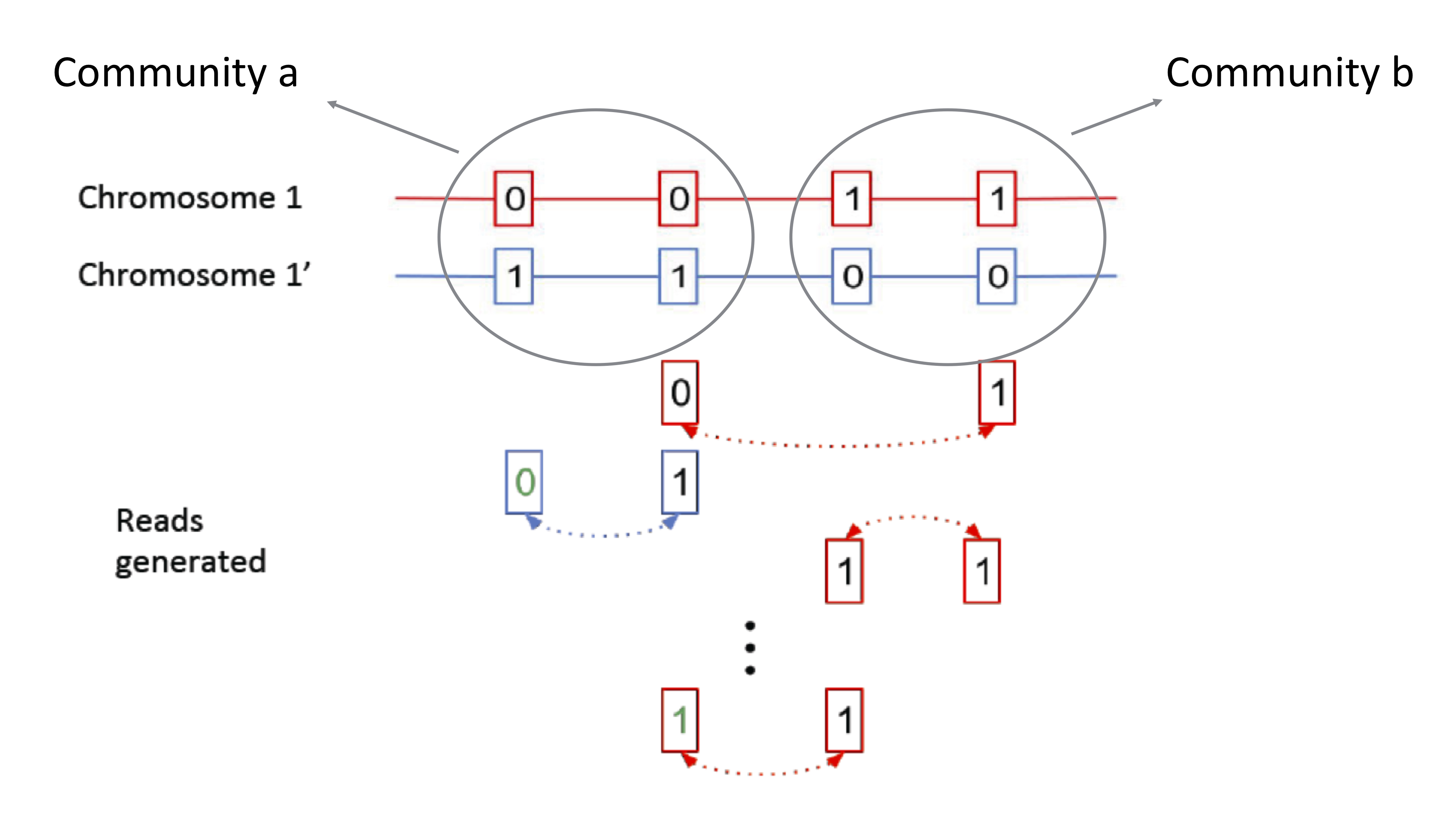
Recall that we are looking at the phasing problem, reformulated as a community recovery problem. The community identity is determined by whether a node is [0 1] or [1 0]. The edges we draw in the graph come from mate-pair reads linking nodes. These parity of these edges tell us the likelihood of whether or not two nodes are in the same community. With 100000 nodes, we need to find an algorithm that’s both accurate and computationally efficient.

Haplotype phasing as a community recovery problem.

Computating all possible partitions and finding the links is exponential in the number of nodes. Thus, we would like to take advantage of global information, but we need a more efficient method of computation. The adjacency matrix \(A\) is an equivalent representation of the data where each column and row represents a SNP. This matrix is usually sparse (i.e. many entries are zero). The above example can be represented by the following adjacency matrix:

Each row and column represents a SNP. \(A_{ij} = 1\) indicates that the two SNPs are in the same community, and \(A_{ij} = -1\) indicates the opposite. \(A_{ij} = 0\) indicates no measurement. This adjacency matrix is typically sparse in practice. We need roughly \(n \log n\) reads in order recover the communities (\(n\) indicates the number of nodes). Where is the information we want in terms of this matrix?

We introduced the concept of a uniform linking model where

Additionally, given that \(A_{ij} \neq 0\), then

\(p\) here describes the probability of error. If there are no errors, we would obtain the adjacency matrix

which has rank 1 (each row is a linear combination of the other rows). Can we now extract the community from this matrix? We note that

is an eigenvector of the matrix. The +1, -1 entries of \(v\) exactly tells us the community membership of the nodes. Therefore in the ideal situation (every read sampled once and no noise), then the principal eigenvector (the only eigenvector) recovers the communities for us. This approach (taking the adjacency matrix and computing the principal eigenvector) is called the spectral algorithm.

The sampling plus the noise adds some randomness to this matrix. Because the randomness is unbiased, we can take the expectation of this matrix, which exactly equals the above matrix in the no noise case. Therefore we are hoping that as we get more data, the estimated adjacency matrix will be close to the expectation of the matrix, which exactly gives us the community membership information.

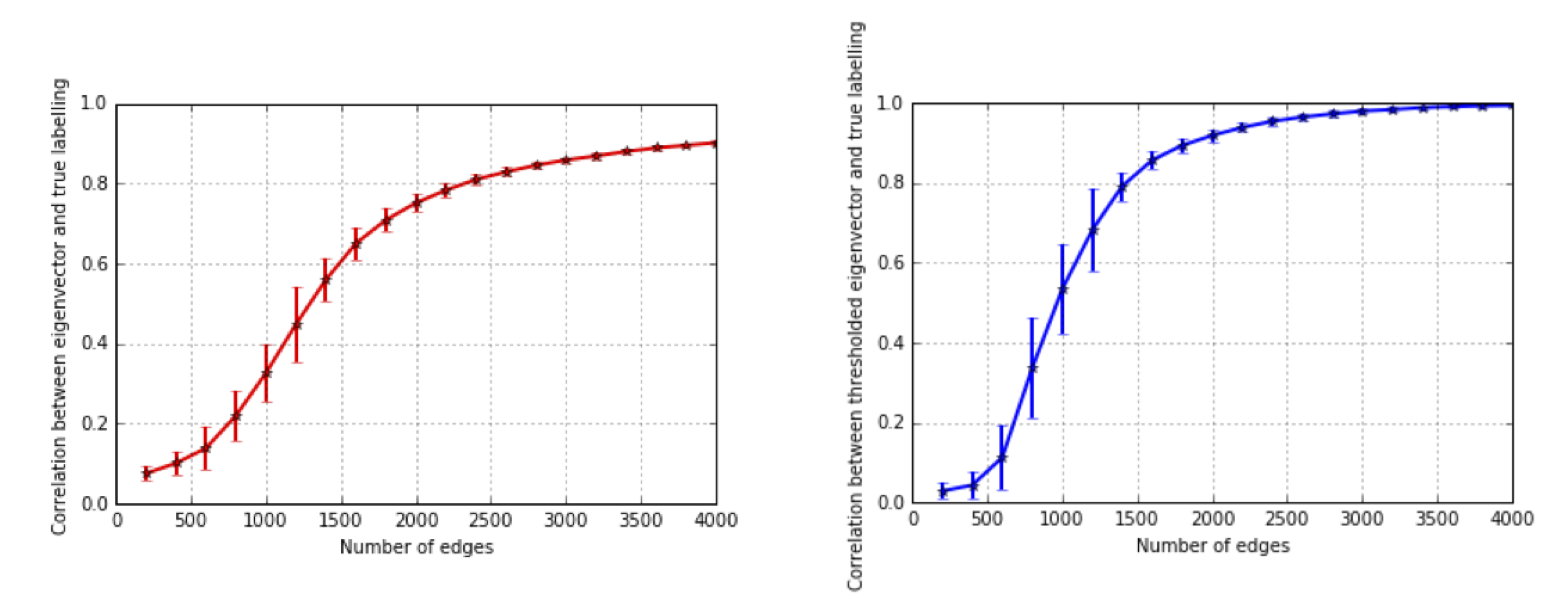
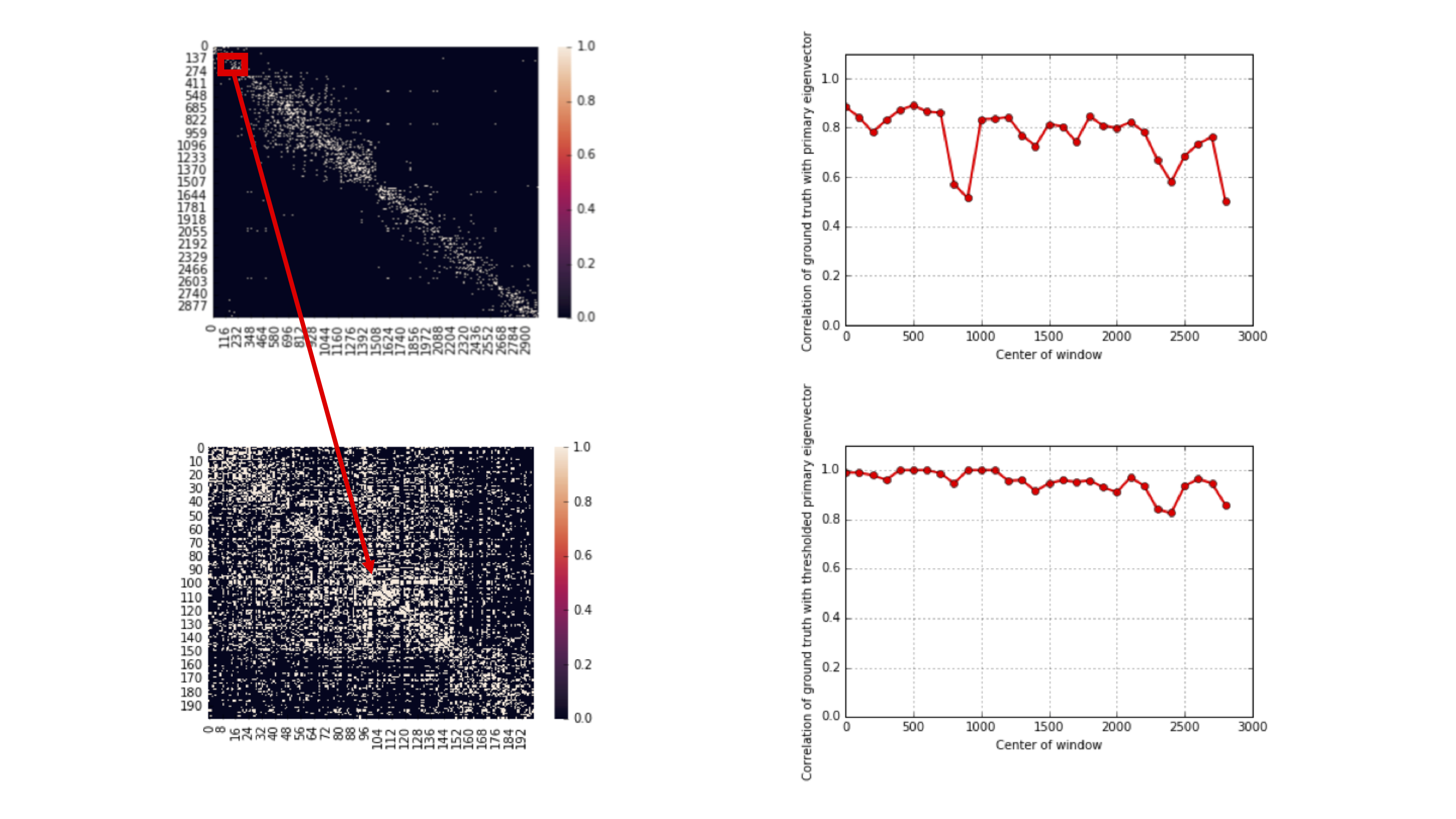
We want to study how the recovered matrix concentrates around the true mean, and the following plot shows how as we increase the amount of data, the recovered principal eigenvector becomes increasingly aligned with the true node membership. Even in a sparse graph, the spectral algorithm is already quite accurate. Note how the recovery scales with the number of edges.

The recovered principal eigenvector concentrating on the true principal eigenvector as the number of edges increases (left: recovered eigenvector, right: thresholeded recovered eigenvector).

Genie-aided lower bound

We want to compute a lower bound on the number of reads required to produce a correct result. Suppose a genie told us the correct community of all SNPs except one (the blue node):

Genie tells us communities of all SNPs expect one.

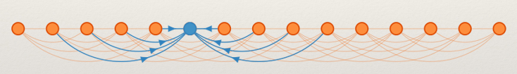
It is still possible to make a mistake if the majority of the linking reads are wrong. A lower bound can be obtained to show that :

where \(D(p||q)\\) represents the binary Kullback-Liebler divergence.

Spectral-Stitching Algorithm

We introduce a two-step algorithm:

1. Approximate recovery using spectral algorithm
2. Refinement using majority vote per SNP

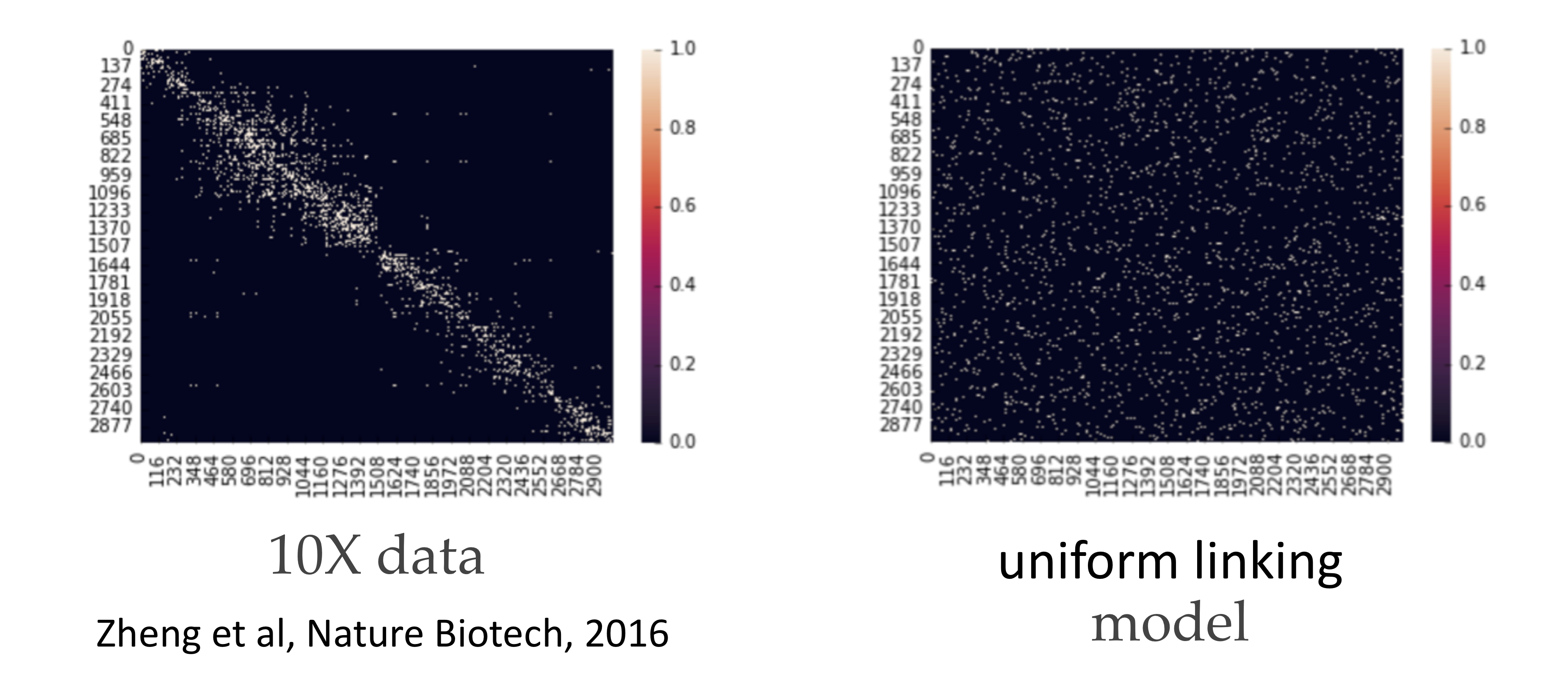
This algorithm actually achieves the lower bound repeated above. 10X genomics provides technology that generates linking information for these SNPs. In this case, the adjacency matrix is also known as a contact map because it tells you the contact information between SNPs. Notably, the adjacency matrix generated from a uniform linking model is quite different from the contact map estimated from a real dataset. This is because in reality, the technology generating the linking information has some limitations, and SNPs that are closer together are more likely to be linked.

The contact map obtained on real 10X data in comparison to the contact map obtained from data sampled from the uniform linking model.

It turns out that if we zoom in on the diagonal, we notice that locally, the matrix appears more consistent with the uniform linking model. Performing the spectral algorithm within these diagonals results in much better recovery:

Motivation for a sliding window/stitching spectral algorithm (top right: recovered eigenvector, bottom right: thresholded recovered eigenvector).

We need to also stitch together the block-wise results to get the membership of all nodes. This motivates the spectral-stitching algorithm:

1. Approximate recovery on overlapping blocks via the spectral algorithm
2. Stitch across blocks
3. Take the majority vote for each SNP.

The algorithm used by 10X is similar in flavor to Viterbi decoding. Because the state-space is very large, a complete exhaustive search is too expensive. The 10X algorithm uses branching and bounding to heuristically get some solution. We note that it’s almost impossible in reality to phase the chromosome because some regions have very few SNPs, and no linking read will capture the information here.

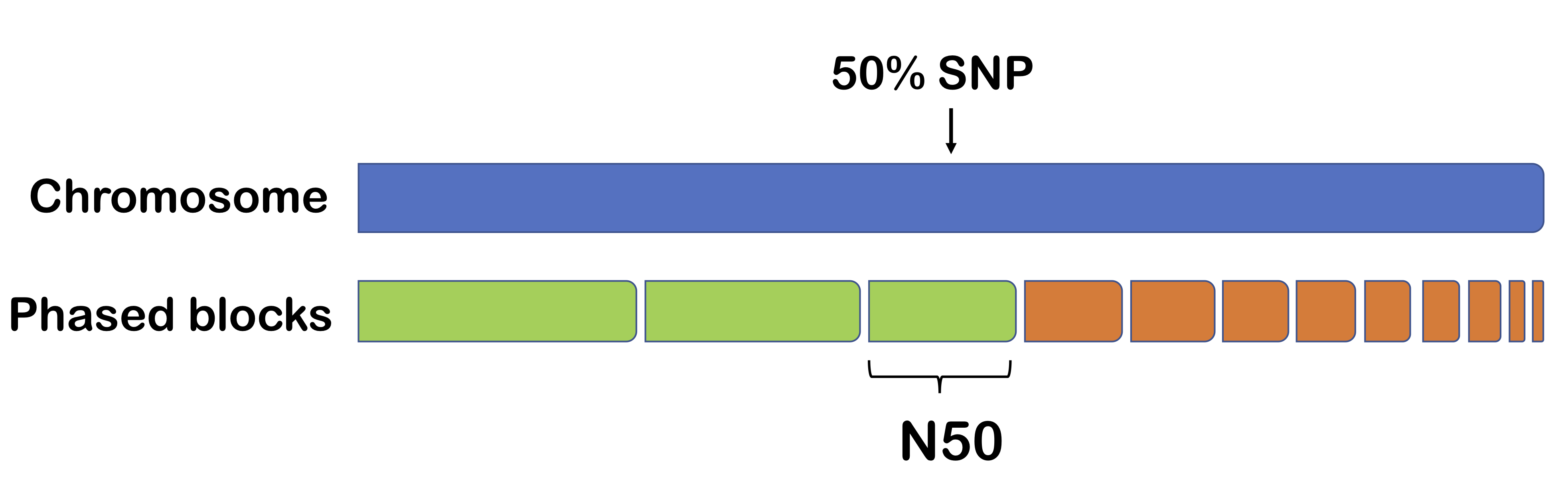
One method for measuring phasing performance is N50. The output of a phasing algorithm is typically in the form of phased blocks (regions of high confidence). Supposed we organize these blocks from longest to shortest. Then N50 is the length of the block such that half the chromosome is contained by the end of the block.

Visual definition of the N50 phasing metric.

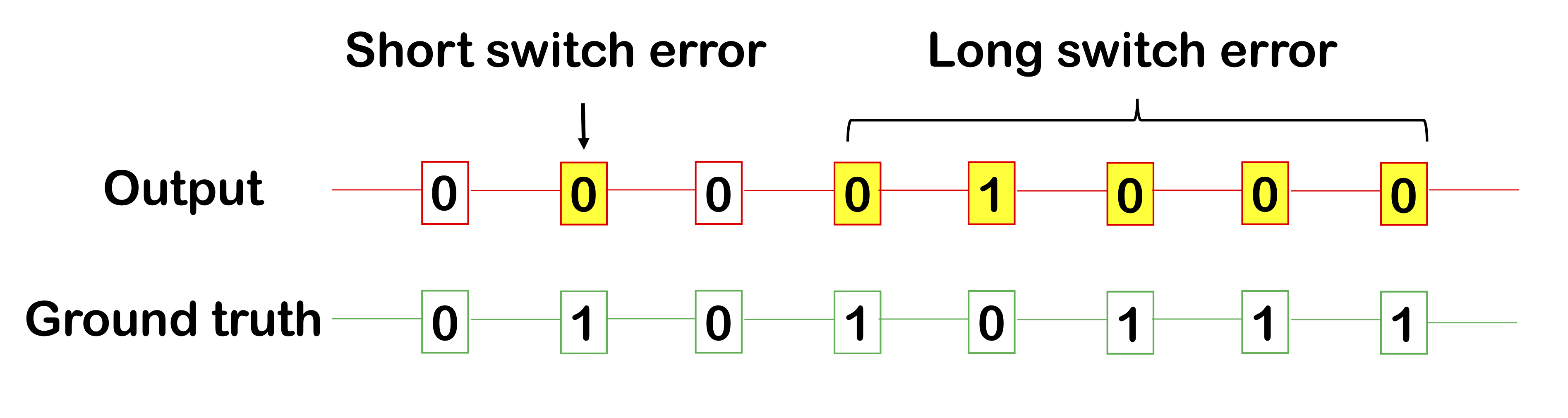
Another method for measuring phasing performance are switch errors within a phased block. We occasionally make some errors within a block, either a short switch error (e.g. 1 SNP) and a long switch error (a long continuous segment of incorrect calls). Intuitively, a long switch error of length, say, 10, should not be worth 10 short switch errors, which is why reporting both these types of errors are useful.

Switch errors that can happen within a phased block.

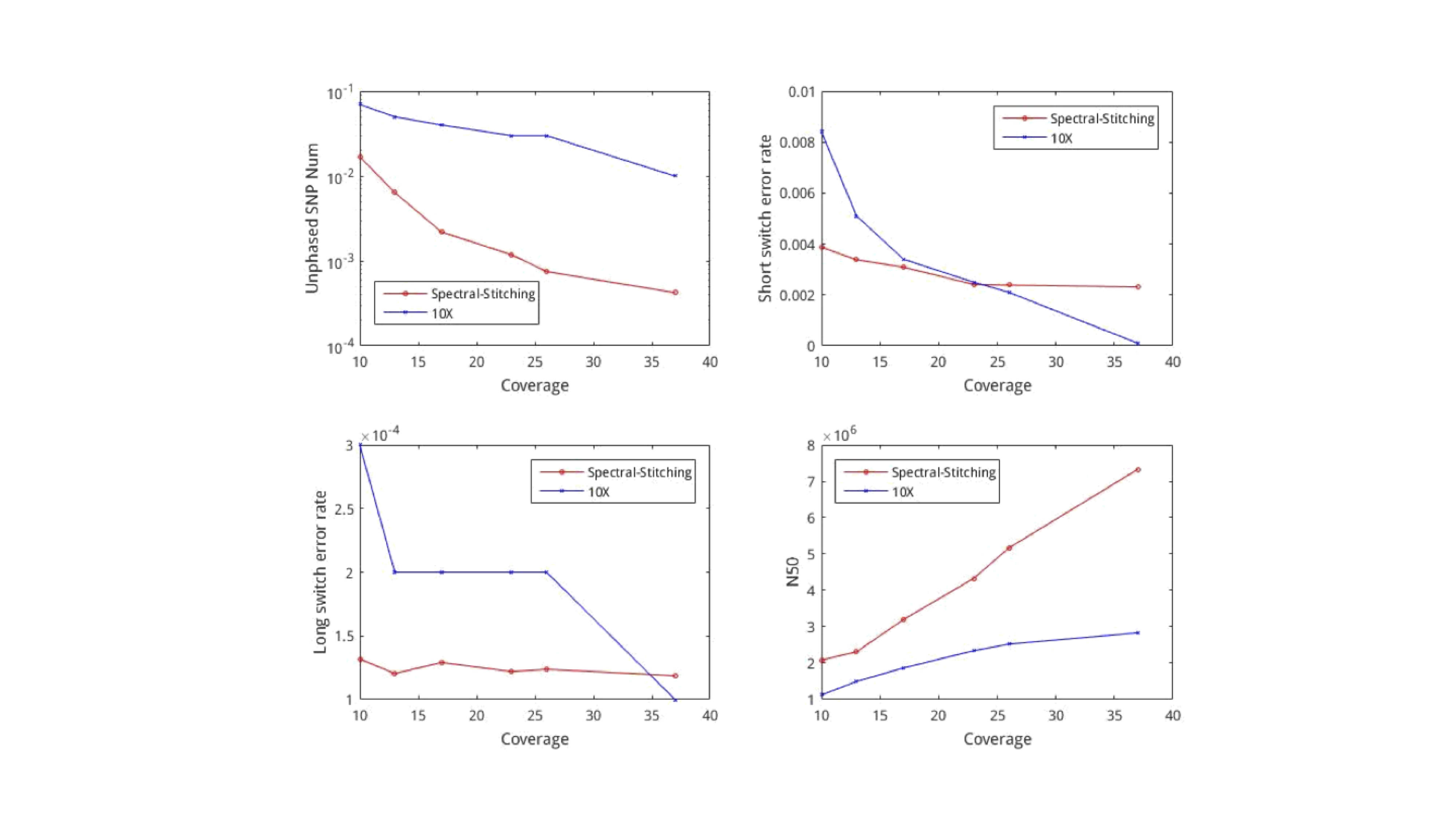
We see that with lower coverage, spectral stitching performs better than the 10X algorithm for all metrics. We note that the algorithm requires about 5500 seconds to process the entire human genome. This is relatively fast, because computing the principal eigenvector can be done cheaply even for large matrices using the spectral method.

Performance of spectral-stitching algorithm on 10X data in comparison to 10X's algorithm.

RNA-seq

So far, all the material covered in this course has revolved around working with data from DNA. From high school biology, you might recall something called the central dogma of molecular biology, an illustrative (but very oversimplified) diagram of how genetic information flows within an organism.

The central dogma of molecular biology.

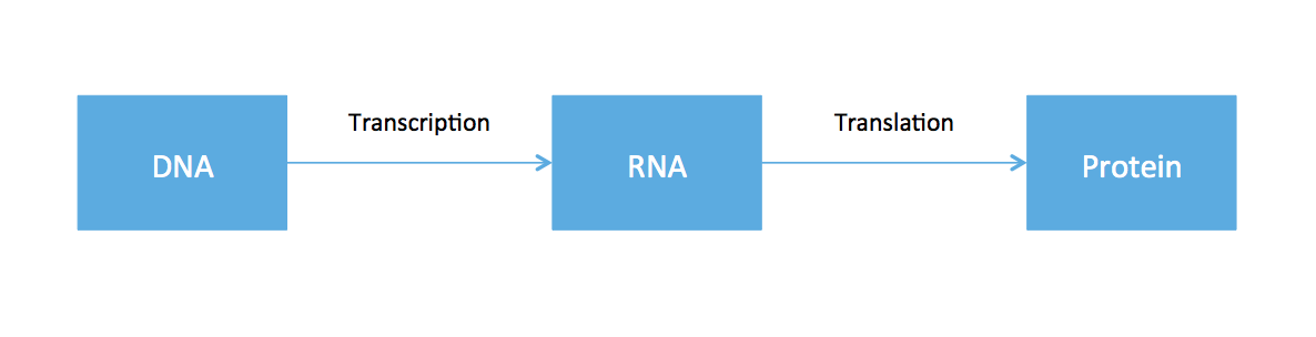
The cell functions by using DNA as the blue-print to to create proteins. Ribonucleic acid (RNA) is produced as an intermediate product. While every cell in the body has roughly the same DNA, cells in different tissues clearly have varying functions. This is because different cells express different RNA. Therefore if one is interested in the dynamics of different cell types, one should somehow measure RNA. While DNA is static, RNA expression can be different depending on time, tissue, and environmental factors.

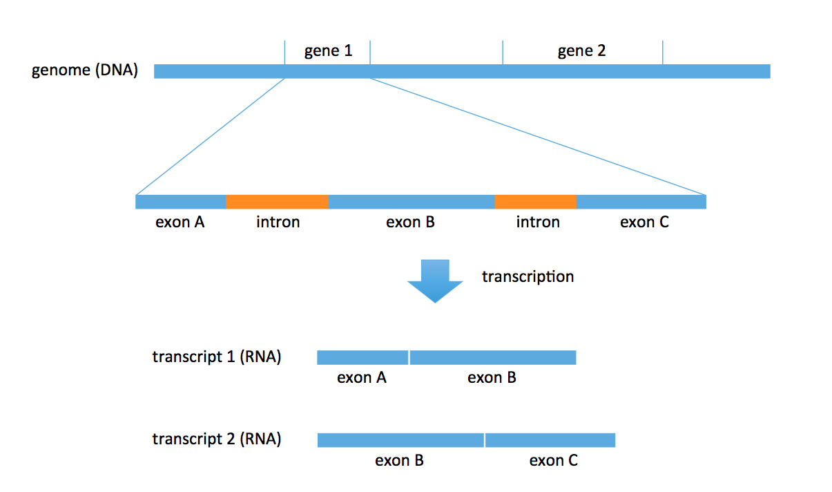
DNA consists of two parts: coding and noncoding. The coding part includes objects called genes. There are roughly 27000 annotated genes in humans, occupying about 1% of the entire genome. A lot of biology revolves around these genes; for example, RNA is transcribed from these genes. Each gene also consists of multiple parts: exons and introns. In the transcription problem, we take a subset of these exons to form an RNA transcript. We could obtain multiple transcripts from the same gene. In the figure below, we obtain 2 distinct transcripts from gene 1, a transcript consisting of exons A and B, and another transcript consisting of exons B and C.

Transcription of genes into RNA transcripts.

There are known genes for which there are 1000s of different types of transcripts (for example, neurexin) produced by the gene. Most genes produce 5-10 versions of transcripts (or isoforms). Transcripts are typically 1000-20000 bp long.

For a given cell, some genes may be expressed and others may not be expressed. The genes that get expressed may have 1 or more isoforms, and each isoform may be expressed in different abundances. Within a cell, we may see tens of thousand of transcripts from the union of all the genes.
A biologist would be interested in identifying these transcripts. Estimating gene expression is the problem of figuring out which transcripts are expressed and at what abundance.

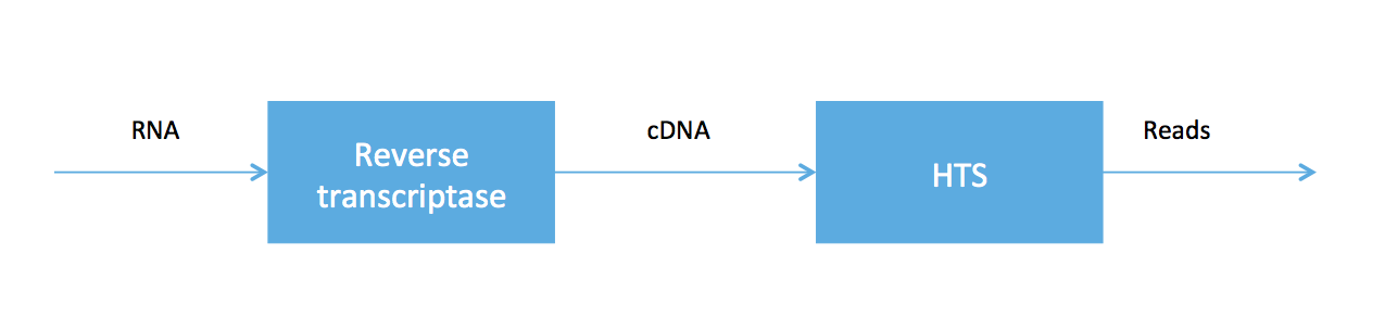
As we said at the beginning of the course, high-throughput sequencing (HTS) is very useful because HTS technologies can be applied to measure other molecules. In RNA-seq, we sample a tissue and, after some chemistry, obtain a soup of RNA transcripts. Biologists have been able to convert the RNA to a special type of DNA (called cDNA) using an enzyme called reverse transcriptase, and we can feed the DNA into our high-throughput sequencer. The pipeline is summarized in the figure below.

The RNA-seq pipeline.

RNA-seq was developed in Mortazavi et. al., 2008. We will focus on computational problems related to getting short reads (100 bp Illumina reads, for example) for RNA-seq.

A counting problem

Let’s say we have two transcripts that appear in different abundances. We get reads randomly from the two transcripts but proportionally to their abundances. We want to infer which transcripts are present and what their abundances are. There are multiple flavours of the problem (listed in order of increasing difficulty):

1. Transcripts are known but the abundances are not.
2. Neither transcripts nor abundances are known. The genome is known.
3. Neither transcripts nor abundances are known. The genome is also not known.

We may encounter the first case if we are working with a popular organism such as a human or mouse. In this case, there exists a curated set of transcripts called the transcriptome. Additionally, different tissues will have different abundances, and this information is the subject of differential analysis. We may encounter the second case if we are looking at an organism whose transcriptome is not known, or cancerous tissue (where the transcriptome is changed by change in genome, but all transcripts seen are reasonably long sequences from the original genome stitched together).

We will start with the first formulation. The computational problem here is a counting problem: we want to count how many reads came from each transcript. Mapping reads to transcripts can be done using various alignment algorithms, which we’ve discussed in previous lectures. Notice that there is an intrinsic ambiguity here: in some cases, one does not know where a read comes from. For example, consider transcripts 1 and 2 in the figure above. If we obtain a read that aligns to exon B, then we cannot tell which transcript it came from. This is an inference problem. Most ambiguities result from different transcripts sharing exons. For simplicity, we currently will not worry about the different lengths of transcripts (this is easy to account for later).

In summary, we have two types of reads: uniquely mapped and multi-mapped. The processing of Mortazavi et. al., 2008 just used the uniquely mapped reads to do inference.

Let \(t_i, \dots, t_k\) be \(k\) transcripts and \(\rho = (\rho_1, \dots, \rho_k)^T\) be the abundances of the transcripts. We obtain N reads \(R_1, \dots, R_N\), and we want to estimate \(\rho\). Let \(N_k\) be the number of reads that map uniquely to transcript \(k\) and \(N = \sum_k N_k\) be the total number of unique reads. Let

In the above example, if we had a third transcript that consists of only exon A, then no part of its sequence would be unique. Therefore the approach of Mortazavi et. al., 2008 will not see any reads from this transcript and we will always obtain an abundance of 0.

Alternatively, we can assign partial counts. In the above example with two transcripts, if we obtain a read that aligns to exon B, we can give half a count to each transcript. This also has its own issues. For example, if the underlying truth is \(\rho_1 = 1\) and \(\rho_2 = 0\), then only transcript 1 is expressed. This scheme will not give us an estimate of 0 for transcript 2. We will address this problem in the next lecture.