Lecture 10: Haplotype Phasing - Community Recovery
Lecture 10: Haplotype Phasing - Community Recovery
Thursday 8 February 2018
Topics
SNP calling
Single Nucleotide Polymorphisms (SNPs) are mutations that occur over evolution. A simplistic view of these would be to think of them as around 100,000 positions where variation occurs in the human genome.
SNP calling is a technique that is used to identify SNPs in the sample genome. The main computational approach taken here is given reads from a genome, we first map the reads to various positions on the genome using alignment methods discussed in the last lecture. Some reads map into locations with no variation with respect to the reference.
At a high level, the pipeline can be seen as follows:
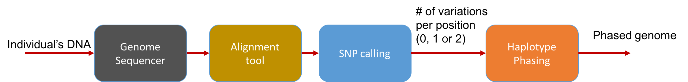
The main statistical problem is to be able to distinguish errors in reads from truly different SNPs in the underlying genome. In practice, we usually have very high coverage; every position in the genome is covered by many reads. Thus we can run a simple statistical test to see if a read disagreeing with the reference is due to errors or due to the individual’s genome actually being different.
SNP calling in diploid organisms
If an organism had only one copy of every chromosome, the SNP calling problem would reduce to just taking the majority of the base of reads aligned to every position. Humans, however, are diploid. They have two copies of every chromosome: one maternal and the other paternal.
During sequencing, we fragment the DNA material, so the sequencer cannot distinguish between the paternal and maternal DNA. When we map each read to the reference sequence, we know its location on the genome but we don’t know whether it comes from the maternal or the paternal chromosome. We represent variation in each position as a 1 and no variation as a 0. In each position, we have 4 possibilities:
- 00 (no variation)
- 11 (both copies are different from the reference)
- 10 or 01 (one of the copies is the reference and the other is the variation)
We note that we assume here that there is only one variant at each position. This is a reasonable approximation to reality.
Positions with 00 and 11 are called homozygous positions. Positions with 10 or 01 are called heterozygous positions. We note that the reference genome is neither the paternal nor the maternal genome but the genome of an un-related human (or more precisely the mixture of genomes of a few individuals). An individual’s haplotype is the set of variations in that individual’s chromosomes. We note that as any two human haplotypes are 99.9% similar, the mapping problem can be solved quite easily.
After mapping the reads, we gain information about the likelihood of four above possibilities. For SNP calling, we can measure (estimate) the number of variations at each position: 0, 1, or 2. Note that we cannot tell between the two heterozygous cases (01 vs 10). Distinguishing these two is important because many diseases are multiallelic. That is, multiple positions determine a disease. Also the diseases depend upon the proteins produced in an individual. This depends upon the SNPs being present on the same chromosome rather than being present on different chromosomes.
Haplotype Phasing
Haplotype phasing is the problem of inferring information about an individual’s haplotype. To solve this problem, there are many methods.
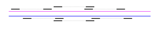
First, we discuss what kind of data is needed to perform phasing. Let’s say we have two variants, SNP1 and SNP2. The distance between the two are on the order of \(\approx\) 1000 bp (i.e. they’re pretty far apart). To do haplotype phasing, one needs some information that allows us to connect the two SNPs so that one can infer which variants lie on the same chromosome. If you do not have a single read that spans the two positions, then you don’t have any information about the connection between the two SNPs.
Illumina reads are typically 100-200bp long and are therefore too short; however, there does exist multiple technologies that provide this long-range information:
-
Mate-pair reads - With a special library preparation step, one can get pairs of reads that we know come from the same chromosome but are far apart. They can be ~1000 bp apart, and we know the distribution of the separation.
-
Read clouds - Pioneered by 10x Genomics, this relatively new library preparation technique uses barcodes to label reads and is designed such that reads with the same barcode come from the same chromosome. The set of reads with the same barcode is called a read cloud. Each read cloud consists of a few hundred reads that are from a length 50k-100k segment of the genome.
-
Long reads - Discussed in previous lectures.
For both of these technologies, the separation between linked reads is a random variable, but one can compute it by aligning the reads to a reference.
In practice, the main software used for haplotype phasing are HapCompass and HapCut. HapCut poses haplotype phasing as a max-cut problem and solves it using heuristics. HapCompass on the other hand constructs a graph where each node is a SNP and each edge indicates that two SNP values are seen in the same read. HapCompass then solves the haplotype phasing problem by finding max-weight spanning trees on the graph. For read clouds, a 10x Genomics’s loupe software visualizes read clouds from NA12878, a human cell line with a genome frequently used as a reference in computational experiments.
The Computational Problem
Here we consider a simplified version of the haplotype phasing problem. We assume we have the locations of the heterozygous positions in the genome, and we only consider reads linking these positions.
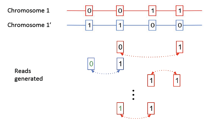
The above figure shows two chromosomes with heterozygote SNPs; we want to identify which variations occurred on the same chromosome. Note that errors can occur in the mate-pair reads, as shown above, resulting in erroneous SNP calls. We will show that the haplotype phasing problem can be cast as a community recovery problem.
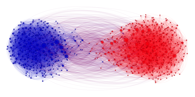
Community recovery problem
In the community recovery problem, we are given a graph with a bunch of nodes, and each node belongs to one of multiple clusters as shown in the figure below. The recovery problem is to recover the clusters (colors) based on the edge information between nodes. This problem is commonly seen in social networks where nodes can be blog posts, for example, and we want to identify which posts are from Republicans and which are from Democrats. The edges describe how the posts link to one another.
Returning to our haplotype phasing problem, we can define each index as a node in a graph. This results in four nodes corresponding to the 4 heterozygous SNP locations. We can also define two communities \(A\) and \(B\) for our graph:
\[A = \begin{bmatrix} 0 \\ 1 \end{bmatrix} \ \ \ \ \ \ \ B = \begin{bmatrix} 1 \\ 0 \end{bmatrix}\]SNPs 1 and 2 belong to community \(A\), and SNPs 3 and 4 belong to community \(B\). In practice, we may have 100,000 nodes with half in each community.A mate-pair read linking two nodes results in an edge between those two nodes, and the weight of the edge depends on the parity of the read. We will show that recovering the communities is equivalent to solving the haplotype phasing problem. The partition will give us all the information except for 1 bit: which SNPs correspond to the maternal chromosome.
A necessary condition for successful haplotype phasing is connectedness; each node has a path to each other node. If there are no errors on the reads, we can recover the communities using a greedy algorithm. We can start at an arbitrary node, assign it to community \(A\), then follow an edge leaving the node. If the edge has weight 1 (indicating that the two nodes are identical), then we assign the next node to community \(A\) as well. Otherwise, we assign it to community \(B\). Note that we can only resolve the nodes into two communities. Without additional information, we cannot know which community corresponds to which chromosome.
However, the above approach is not robust to errors in the reads: once there is a single error in a read, the algorithm will make mistakes on the communities of the subsequent nodes that the algorithm visits. An alternative global approach for finding the communities would be to enumerate all possible pairs of communities. We would then simply choose the solution that results in the maximum likelihood given the data. This algorithm can be reduced to the MAXCUT problem, which is NP-hard.
To seek an alternative algorithm that is more efficient and yet robust, we will first assume a uniform linking model; reads are equally likely to be between any pair of SNPs. For our haplotype example, we can construct the adjacency matrix
\[A = \begin{bmatrix} \star & -1 & 0 & 0 \\ -1 & \star & 1 & -1 \\ 0 & 1 & \star & 1 \\ 0 & -1 & 1 & \star \end{bmatrix}\]where position \(A_{ij} = 1\) if the SNPs at indices \(i, j\) are equal. Otherwise, \(A_{ij} = -1\). This matrix captures all the information in the graph. We claim that the communities can be extracted efficiently from this matrix under the uniform linking model. We will explore this further next lecture.