Lecture 1: Introduction
Lecture 1: Introduction
Tuesday 9 January 2018
Topics
What is high-throughput sequencing?
The main object of interest in this course is the genome of a organism, which is made of deoxyribonucleic acid (DNA). All computational methods we discuss will be related to deducing the sequence of the genome or some property closely related to the genome. High-throughput sequencing (HTS) refers to modern technologies used to identify the sequence of a segment (or “strand”) of DNA. Only 17 years ago, sequencing technologies were around 6 orders of magnitude slower than they are today in terms of both cost and throughput.
The first major sequencing project was the Human Genome Project. A big consortium began collaborative efforts in 1990 to sequence the entire human genome. The project was nominally completed in 2003, costing $2.7 billion and 13 years of work by labs around the world. In 2017, the cost of sequencing a genome was approximately $1000. This is testament to how far the technology has evolved. As shown below, the cost of DNA sequencing has been falling at a rate faster than Moore’s law over the last 17 years.
DNA is a very important biomolecule, but it’s only one of many important biomolecules. Other important biological molecules include ribonucleic acids (RNA) and proteins. Some innovative bio-chemistry has allowed the use of DNA sequencing technology for measuring properties of various other biological molecules (and there are even proposals on how to use DNA sequencing for detecting dark matter).
HTS can be thought of as a microscope that can be used to measure a variety of quantities. The basic paradigm (shown below) is to reduce the estimation problem of interest to a DNA sequencing problem, which can be handled using HTS. This is similar in principle to the reduction used to solve many mathematical problems or to show NP-hardness of various problems.
To get a sense of the scale of the data, consider the human genome \(G\) which consists of 3 billion bases \(\{A, C, T, G\}\). Suppose each read has a length \(L\) of 100 bases. The coverage depth is the average number of reads that cover a given base in the genome. To achieve a coverage depth \(C\) of 30x, we would need \(N=900,000,000\) reads since \(C = NL/G\). Therefore any algorithm that runs superlinearly in the amount of data will take too long for practical purposes here. In this course, when we say low complexity v. high complexity, we are really talking about linear v. nonlinear.
For the biochemist, the challenge is in determining how to convert the problem of interest to a problem which can be tackled using HTS. This is similar to how biologists design experiments such that the results can be observed under a microscope. For the computational biologist, the challenge is in performing the relevant type of inference on the data observed using HTS. Some important sequencing assays are:
- RNA-Seq: RNA is an important intermediate product for producing protein from DNA. While every cell in an organism has the same DNA, an individual cell’s RNA content may be very different. RNA in cells can also vary depending on temporal and environmental factors. RNA-Seq is an assay that “measures” RNA, and this was the first assay in which HTS was used to measure a molecule other than DNA. The assay was developed in 2008 by Mortazavi et al.
- ChIP-Seq: Different cells express different RNA because of epigenetic factors or molecules that influence how the genome is packed in the cell. DNA in cells are bound to proteins called histones, and for different cells, different parts of the genome are bound to histones. DNA wrapped around histones are harder to access and are not converted to RNA. ChIP-Seq is an assay which was developed measure the regions of the genome that are bound to histones. This assay was developed in 2007 by Johnson et al.. Another recent assay called ATAC-seq measures regions of the genome that are not bound to histones.
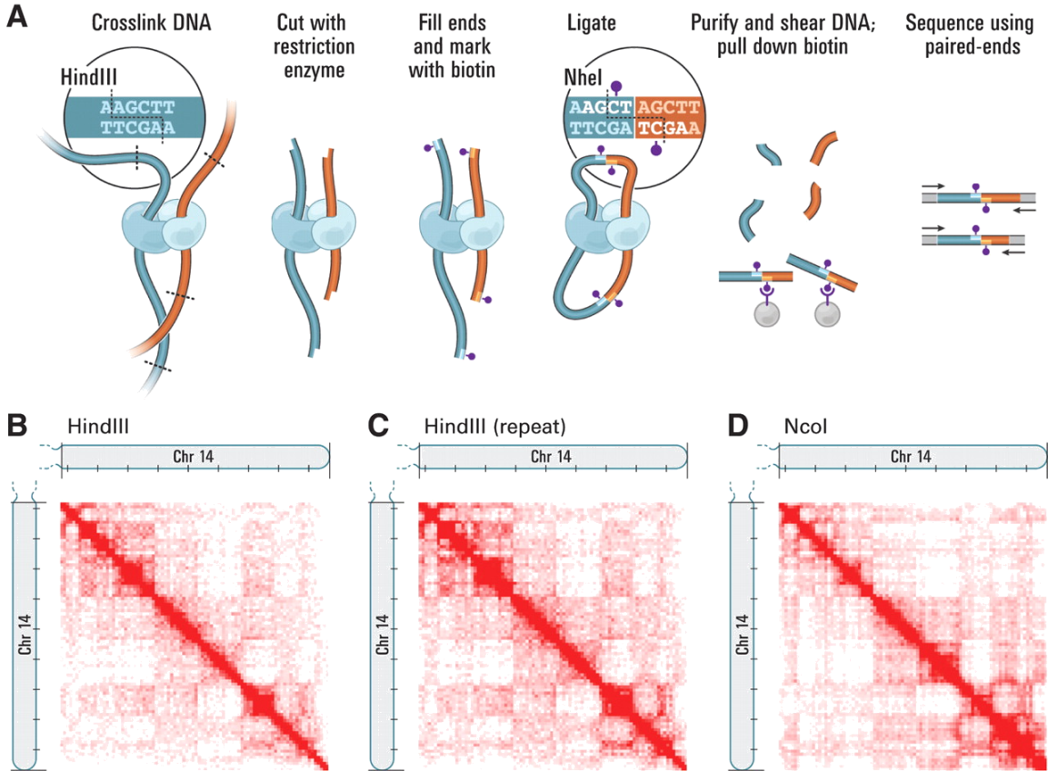
- Hi-C-Seq: This assay measures the 3D structure of molecules and was developed by Belton et al. in 2012.
One of the most interesting and important problems in genomics is predicting phenotype (physical characteristics such as a person’s height or a person’s favorite color) from genotype (DNA sequence). In medicine, understanding the relationship between phenotype and genotype can allow researchers to predict a patient’s susceptibility to certain diseases by sequencing the patient’s genome. A big success-story here is the discovery that presence of a particular mutation in the gene BRCA1 increases the risk of breast cancer to around 45%.
Another important application of HTS is cancer. Cancer is a “disease of the genome.” It is caused by rearrangements of the genome, which are sometimes very large. By sequencing cancer cells, one gets information about the nature of the cancer-causing mutation and can tailor treatment.
Non-invasive pre-natal testing for genetic birth defects is another powerful application of HTS. Traces of fetal DNA can be found in the blood of the mother. The main idea here is to sequence the maternal blood and infer fetal genetic birth defects from the sequence. HTS has been used successfully for detecting Down syndrome.
Sequencing methods
Science progresses by the invention of measuring methods. HTS is one such measurement tool; however, HTS is different from many measurement tools because it has a significant computational component. HTS (also called shotgun sequencing) takes the DNA sequence as input, breaks it into smaller fragments or reads, and returns a noisy version of these smaller fragments. We note that the length of reads range from 50-50000 while the human genome is of length 3 billion. Fortunately, these small noisy subsequences also contain information about the genome. While a single read contains very little information about the entire sequencing, a typical experiment generates a few hundred million reads (and hence is called “high-throughput”). Extraction of the information contained within reads requires clever computational processing, and this is the flavor of problems we will discuss in this class. We also note that the sequencing process can be very noisy. Each of the reads can be potentially different from the original subsequence of the DNA the read came from.
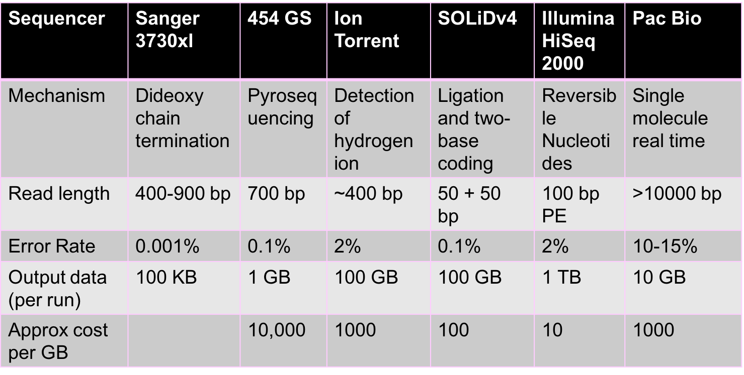
The sequencing revolution arose due to the rapid evolution of sequencing technologies. Sequencing began with Fred Sanger, who first came up with Sanger sequencing technology. This was a relatively low-throughput technology and was the dominant technology until the late 1990s. Second generation sequencing is most heavily represented by Illumina and is currently the dominant technology. Recent developments in Illumina sequencing have allowed scientists perform single-cell sequencing or the sequencing of individual cells. Companies like PacBio and Oxford Nanopore have led recent developments in third and fourth generation sequencing technologies.
HTS is a fast changing area with new technologies emerging constantly. All these technologies give us reads, but each uses different chemical processes to generate the reads. There are two main properties of reads that are important from a computational perspective:
- Read lengths: The longer the reads are the more information they contain. Ideally, a read is simply the entire genome. Unfortunately, a read of such length is not achievable by chemistry today or in the foreseeable future. Illumina reads are around 100bp-200bp long, and PacBio reads are over 10000 bp long. While PacBio reads are longer than Illumina reads, they are still much shorter than genome lengths.
- Error rates and types of errors: Illumina has relatively low error rates of 1-2%, and errors here are mostly substitution errors (i.e. a base being replaced by some other base). PacBio reads have higher error rates of 10-15%, and errors here are insertions and deletions.
The figure below shows some characteristics of different sequencing technologies.
EE 372: Data science for HTS
The success of HTS is mainly due to the creative use of read data to solve various problems. For this course, data science problems can be categorized into one of three types:
- Data processing:
- Assembly or de novo assembly: Recovering the DNA or RNA from short noisy reads.
- Variant calling: Individuals of the same species have very similar genomes. For example, any two humans share 99.8% of their genetic material. Because a reference human genome is available, scientists are often interested in the differences of an individual’s genome from this reference genome. Variant calling is the problem of inferring these differences.
- Phasing: The chromosomes in humans (and other higher animals) come in pairs but are crushed and sequenced together. Often scientists want to separate the sequence on the two chromosomes. This is called the phasing problem.
- Quantification: RNA is an important biological molecule in cells, as discussed above. There are potentially 10000s types of RNA molecules observed in an individual cell. Quantification is a counting problem; scientists are interested in estimating how many copies of each type of RNA are in a cell or population of cells.
- Data management: With large databases, natural problems that arise include
- Privacy
- Compression
- Data utilization: Here we use the data to make useful inferences. These problems include
- Single-cell analysis: Properties like diversity in cell populations are inferred from single-cell datasets.
- Genome Wide Association Studies (GWAS): This problem looks at the association between genomes and various characteristics of individuals.
- Multi-omics data analysis: Methods for combining DNA, RNA, and protein measurements to make predictions.
These different problems are illustrated below:

Tools
When working with HTS data, we first attempt to model the data. This usually involves many assumptions which are not true in practice. While inaccurate, these models are used to come up with initial interesting algorithms. As real data often does not satisfy these assumptions, some additional effort is required to get working algorithms even when the modeling is reasonable. Some tools we will use in this course are:
- Combinatorial algorithms: Problems like genome assembly involve working on combinatorial objects like graphs, and combinatorial algorithms naturally follow.
- Statistical Signal Processing: Because the data is noisy, we need signal processing techniques for dealing with the noise.
- Information Theory: When performing inference, this gives a sense of how much data is necessary to achieve “good” estimates, allowing us to design optimal algorithms to achieve such estimates.
- Machine Learning
Objectives
In this course, we will work towards two key objectives:
- Introduce an important and exciting application domain for data science.
- Introduce interesting algorithms and statistical concepts in a concrete well-motivated setting.
Example Problems
In this section, we discuss representative problems that will be covered in this course.
DNA-assembly (de novo)
The DNA sequencer outputs an analog signal (e.g. light intensities or electric signals). We want to process this signal to get the sequence. In essence, one could think of the DNA as a message, the sequencer as a communication channel, and the base caller and assembler as the decoder. This abstraction is shown below:
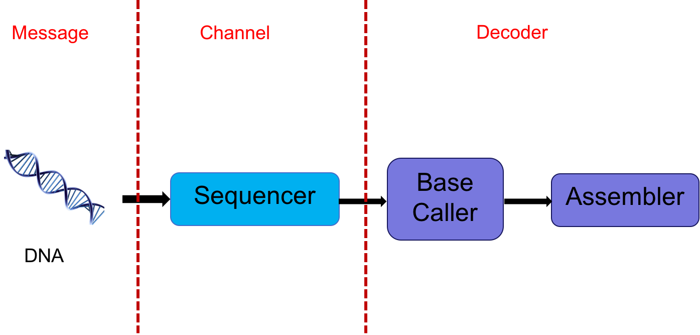
This abstraction gives us multiple avenues of exploring potential problems. The extraction of digital information (discrete bases) from analog signals is a statistical signal processing problem. This involves various stochastic models with many parameters which need to be estimated. Furthermore, one often has to account for signals from adjacent bases interfering with one another. Dealing with intersymbol interference is also a signal processing problem.
We can also consider the problem of assembling the genome from the reads obtained after processing the analog signals. We want to first obtain an estimate of the number of reads necessary to be able to assemble with reasonable accuracy. Using tools from information theory, we can identify bottlenecks and design principles to deal with them, allowing us to design efficient algorithms to overcome these bottlenecks. By efficient here we mean linear in the number of reads. In general, the size of data makes any super-linear algorithm unfeasible in most cases; however, there are cases where smart algorithm design and low level optimized software allows one to use algorithms that are quadratic in the number of reads.
de novo here means “from new,” which is relevant when we assemble a genome for the first item, for example in a new strain of bacteria or in cancer.
DNA Alignment
The alignment problem is as follows: given a reference genome and a new read, we are interested in finding where the new read aligns to the reference genome. This is useful for finding the genomic regions that distinguish two individuals, which may indicate risk for disease and likelihood of possessing certain phenotypes. This problem is nontrivial for three reasons:
- There are errors in the reads, and therefore looking for exact alignment is challenging.
- The genome is quite repetitive, and therefore a read may have several places it can align to. In fact, there are regions of the genome (e.g. Alu repeats) that are repeated millions of times.
- Recall above that we need to align \(N =\) 900,000,000 reads to a length 3B genome. Therefore the naive process of scanning the entire genome for each read’s match is too slow.
RNA quantification and analysis
As discussed above, RNA is another important biological molecule. There exists around 20000-100000 RNA sequences (or transcripts) floating in each cell, each of which are 1000-10000 bp long. Biologists are interested in the problem of quantifying or estimating the number of each RNA transcript (the expression level of that transcript) in a cell.
Biologists and chemists have figured out ways to convert RNA back into DNA (mainly using an enzyme called reverse transcriptase) and then sequence the DNA to get reads using HTS. The computational problem is trying to estimate the number of transcripts of each type from these reads.
One often uses the reference of known transcripts observed in an organism: the transcriptome. Despite there existing a reference, many transcripts have common subsequences and therefore one can not always be sure of where a read originates from. A good algorithm for solving this problem is expectation-maximization (EM).
Downstream analysis
Suppose we measure gene expression levels of two types of mice, for example a stressed mouse v. a relaxed mouse. Based on the expression levels of all 20000 genes, we can ask: which genes distinguish the two mouse states? This problem is known as differential expression.
Additionally, because there are so many genes, by sheer luck, some genes may appear to be significant. To account for this issue, we will leverage techniques from multiple hypothesis testing (e.g. false detection rate control).
In a bulk experiment, a biologist crushes the 100s of millions of cells in a tissue together. After sequencing, the biologist obtains a mixture of the RNA of all cells in the tissue. The transcript counts (or abundances) obtained are therefore an estimate of the sum over all cells. Recent technologies have allowed biologists to sequence biological samples such as tissue at the single-cell resolution. Single-cell technologies allow researchers to observe the diversity of cells within a cell population. Relevant problems here include dimensionality reduction, clustering, and identifying relevant features for characterizing cell types.