Lecture 9: Assembly - Multibridging and Read-Overlap Graphs
Lecture 9: Assembly - Multibridging and Read-Overlap Graphs
Monday 25 April 2016
Scribed by Min Cheol Kim and revised by the course staff
Topics
In the last lecture, we discussed a practical algorithm based on the de Bruijin graph structure. In this lecture, we examine a tweak of the de Bruijin structure (k-mers) that has better performance. We then discuss the notion of read-overlap graphs.
Review of de Bruijin algorithm
de Bruijin Graph Algorithm:
- Chop L-mers (reads) into k-mers, the basic units of the algorithm.
- Build the de Bruijin graph from the k-mers.
- Find the Eulerian Path.
Conditions for de Bruijin to succeed:
- k - 1 > \(\ell_{\text{interleaved}}\) (length of the longest interleaved repeat)
- DNA is k-covered (the reads cover all bases in the DNA, and each read has k-overlap with at least one other read)
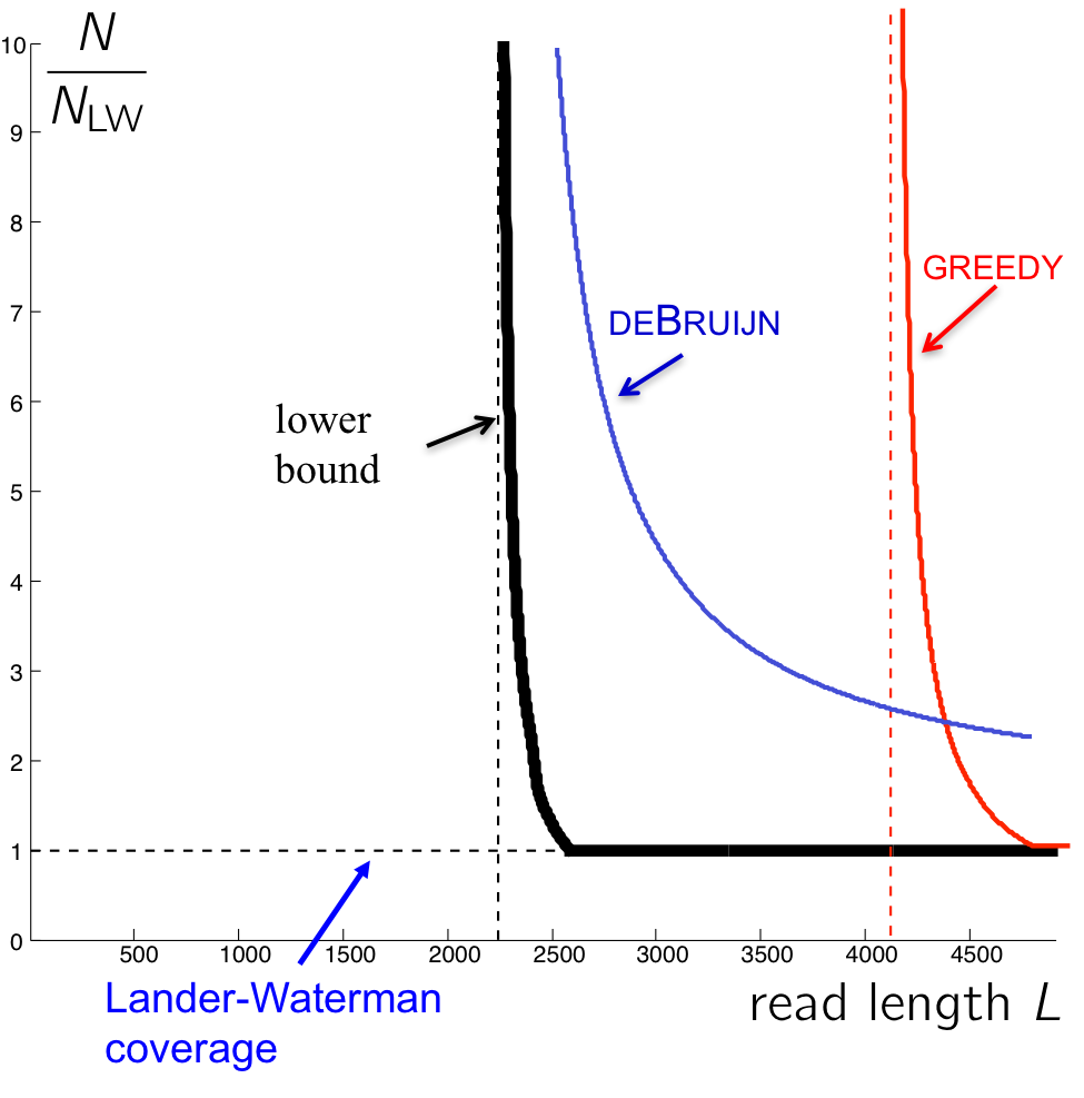
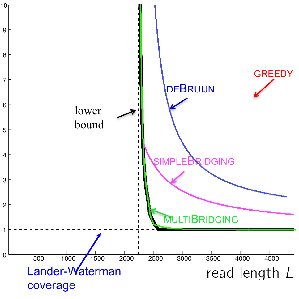
Observe that the de Bruijin graph algorithm can achieve perfect assembly at shorter read lengths than Greedy, but the coverage depth must be very high (even worse than Greedy in some cases!). This comes from the condition on bridging (k - 1 > \(\ell_{\text{interleaved}}\)), which requires that the k-mers must bridge every interleaved repeat.
For the lower bound, the necessary condition for reconstruction is that the interleaved repeats are bridged by the reads (not k-mers). There are only a few long interleaved repeats, and it is overkill to bridge all those with k-mers. We have the information to cover these interleaved repeats with the L-mer (reads) themselves, but we are not using this information by chopping them all into k-mers.
Making k smaller
By taking advantage of the fact that we do not need to bridge all interleaved repeats with k-mers, we can come up with modified versions of the de Bruijin algorithm. We set k \(<< \ \ell_{\text{interleaved}}\), and we do something special for the long interleaved repeats, which are few in numbers.
Simple Bridging
The problem we had when k \(\leq \ell_{\text{interleaved}}\)+ 1 was that we have confusion when finding the Eulerian path when traversing through all the edges, as covered in the previous lecture (Refer to examples of de Bruijin graphs in Lecture 8). When multiple Eulerian paths exist, we cannot guarantee a correct reconstruction.
We can circumvent this problem by using the reads (L-mers) themselves to resolve the conflicts. In the figure below, with k < \(\ell_{\text{interleaved}}\), there were two potential Eulerian paths: one traverses the green segment first and the other traverses the pink segment first.
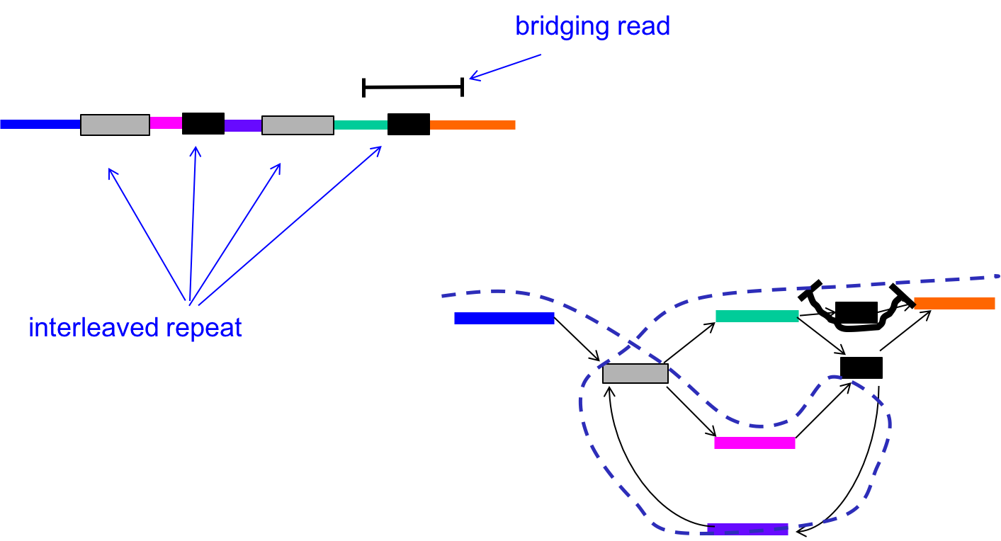
By incorporating the information in the bridging read, however, we can reduce the number of Eulerian paths to one. In other words, we can resolve the ambiguity in the graph as follows:
- Find the bridging read on the graph, in this case on the top right.
- Since we know that the orange segment must follow the green segment, replicate the black node and create a separate green - black - orange path.
Information from bridging reads simplify the graph.
At this point, our conditions for a successful assembly is as follows:
- All interleaved repeats (except triple repeats) are singly bridged.
- k-1 > \(\ell_{\text{triple}}\) (length of the longest triple repeat).
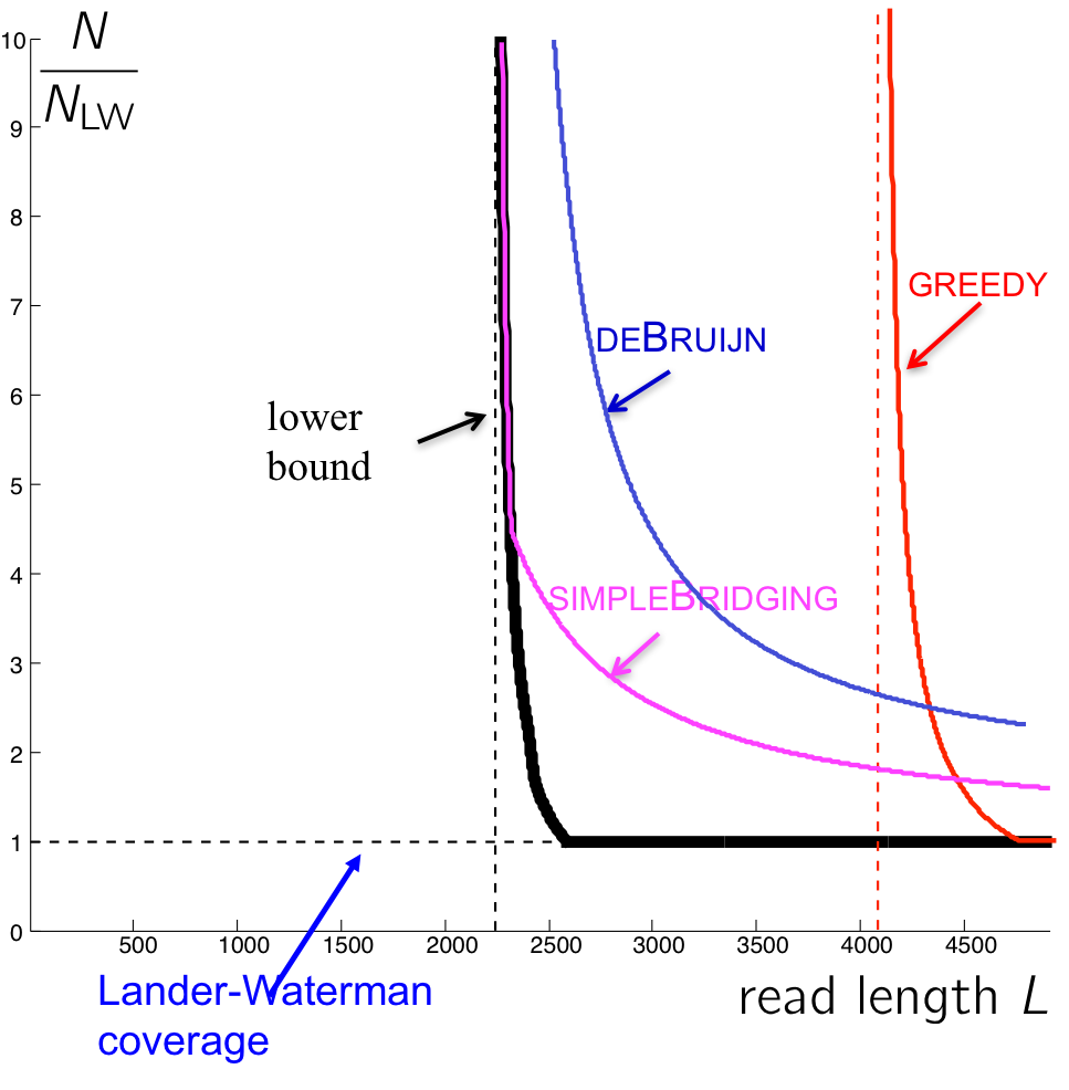
The performance of this algorithm is shown in the figure below. Note that even though this reduces the number of reads we need, it is still not as close to the lower bound as we hope. Can we do better?
Multibridging
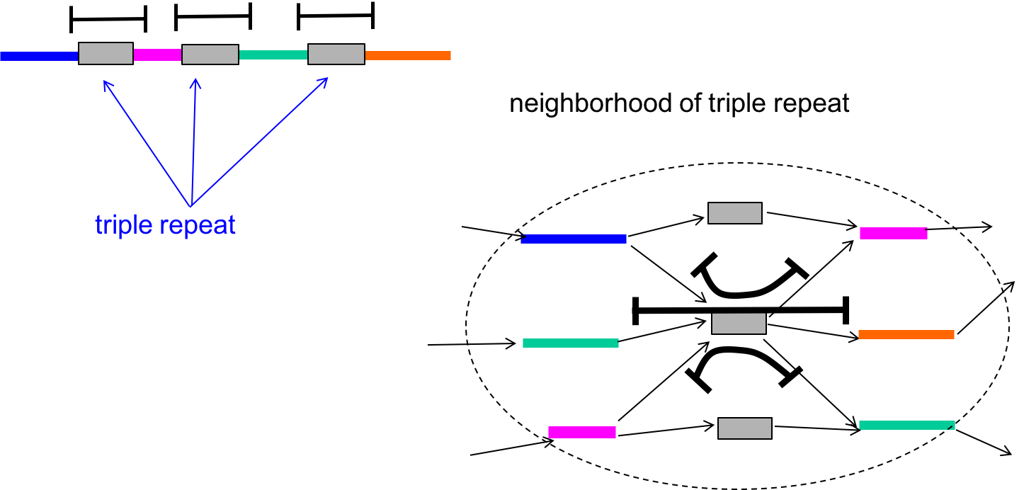
The algorithm we outlined above had k - 1 > \(\ell_{\text{triple}}\) as a condition, which allowed us to guarantee the bridging of all copies of all triple repeats. A triple repeat is a special type of interleaved repeat in that there may still be ambiguity to the Eulerian path even if the repeat is bridged.
We can modify the algorithm further to get around the ambiguity. If the triple repeats are triple-bridged (meaning that every copy of the repeat is bridged by a read), then we can separate the repeat node into three different distinct nodes that each connect to distinct adjacent nodes. This is shown in the figure below.
With this in mind, our conditions for success then becomes (Bresler, Bresler, Tse, 2013):
- All copies of all triple repeats are bridged.
- Interleaved repeats are singly bridged
- Coverage (each base in the genome is covered by at least one read)
We also see that the performance of the multibridging algorithm is close to that of the lower bound.
Assembly problem revisited: read-overlap graphs
So far we have looked at algorithms based on de Bruijin graphs. These algorithms essentially chop reads into shorter k-mers. Then we realized that the k-mers do not contain enough information, and we brought back some of the important reads to resolve conflicts.
This seems like a strange paradigm since the reads are the ones that contain all the information to begin with (why chop them up only to bring them back?). A more natural class of algorithms are based on read-overlap graphs, which is actually the original approach to assembly.
Read-overlap graphs
Instead of thinking about k-mers, we should think about reads themselves. Using this idea, we reconstruct a graph where all the nodes of the graph are reads (without any k-mer transformation). Then, we connect every pair of nodes with an edge, building a complete graph. Each edge is associated with a number that indicates the amount of overlap between the two nodes (reads). Alternatively, we can also associate each edge with a number that indicates how much length we gain by joining the two reads.
An example of a read-length graph is shown below. If you have two reads ACGCA and CGCAT, you would get an extension of 1 (overlap of 4) when the reads are put together to form ACGCAT.
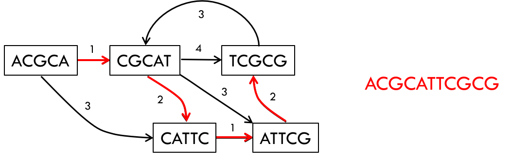
In some sense, this is the most natural representation of the assembly problem. To solve the problem we would take a path that goes through every single node in the graph while also minimizing the sum of the extensions (or maximizing the sum of the overlaps).
This path is called the Generalized Hamiltonian Path, a path that visits every node at least once while maintaining the minimum sum of weights (note the difference between this and the Eulerian path). We may need to visit a node multiple times due to repeats.
It turns out that this problem is NP-hard. This is one of the main motivations for working with the de Bruijn graph instead.
Information limit and solving instances of an NP-hard problem
Under some assumptions, we can solve this problem, which is NP-hard in general.
Let us see what the most basic algorithm does in terms of the read-overlap graph - the Greedy algorithm. For each node, the Greedy algorithm picks the edge with the largest overlap going out, ignoring all other edges for that node. This vastly simplifies the graph with only one outgoing edge from each node.
Greedy’s pitfall is that when the true path visits a node twice, the algorithm will fail. The approach is an oversimplification of the generalized Hamiltonian path problem.
Going back to our performance figure, we see that the Greedy algorithm lives in the red region where the read length is long enough to cover all repeats. That leaves the blue region where reconstruction is still possible but we may need to visit the nodes more than once.
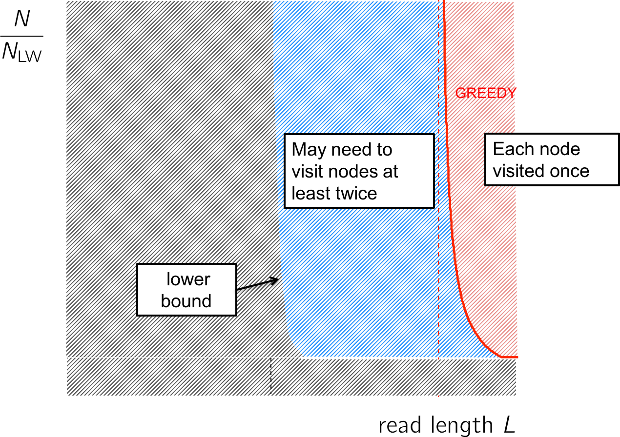
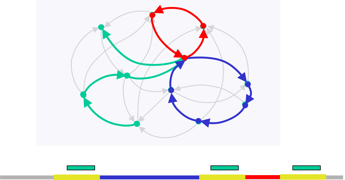
Note that we only need to visit a node more than 2 times if and only if there exists an unbridged triple repeat, but reconstruction in this situation is not possible anyway. In the figure below, we notice that we cannot determine whether we should traverse the blue or red path first.
The information analysis shows us that the Greedy is an oversimplification, but we do not need to visit a node more than twice; this stands on the left of the lower bound (figure below). We need an algorithm that visits each node no more than twice.
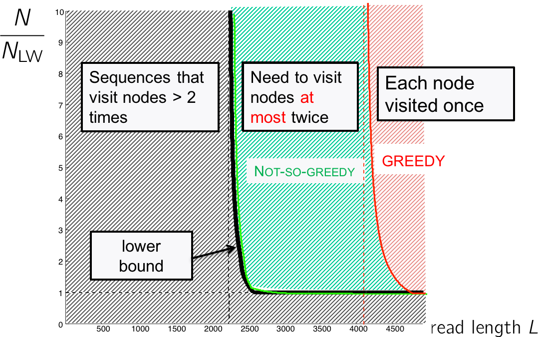
This algorithm is called the “Not-so-greedy” algorithm, and it keeps exactly the two best extensions for each node. The complexity is linear with the number of reads. Therefore in the green region, we can overcome the NP-hardness of the Hamiltonian problem.