Lecture 8: Assembly - The de Bruijn Graph Algorithm
Lecture 8: Assembly - The de Bruijn Graph Algorithm
Wednesday 20 April 2016
Scribed by Renke Pan and revised by the course staff
Topics
Review
Recall that last time we introduced the de Bruijn Graph and the Eulerian Path. A de Bruijn Graph can be constructed from the L-spectrum through the following steps:
-
Add a vertex for each (L-1)-mer in the L-spectrum.
-
Add k edges between two (L-1)-mers if their overlap has length L-2 and the corresponding L-mer that contains both appears k times in the L-spectrum.
An Eulerian Path of a graph is the path that traverses each edge of the graph exactly once. Note that the Eulerian algorithm can find an Eulerian path in linear time. Recall that the greedy algorithm would need to compute overlaps between reads. If done naively this scales quadratically in the number of reads. We will discuss this in the coming lectures.
Here we consider the Dense Read Model, where we assume that a read starts at every base in the genome. This gives us the L-spectrum of the genome. From this, we build a de Bruijn graph as described above. As discussed in the last lecture, every Eulerian path in the de Bruijn graph corresponds to a genome consistent with the data.
In this lecture we will discuss the conditions for the uniqueness of the Eulerian path and hence of the reconstruction of the genome. We will next see a modification of the de Bruijn graph algorithm so that it works on arbitrary reads rather than the L-spectrum of the genome. We will evaluate its performance and look at some refinements.
Examples of de Bruijn
At the end of the last lecture, we stated the following theorem:
Theorem [Ukkonen 1995, Pevzner 1992]: The necessary and sufficient condition for assembly from the L-spectrum of a genome is that L - 1 > \(\ell_{interleaved}\), the length of the longest interleaved repeat of the genome.
We see this by a few examples here.
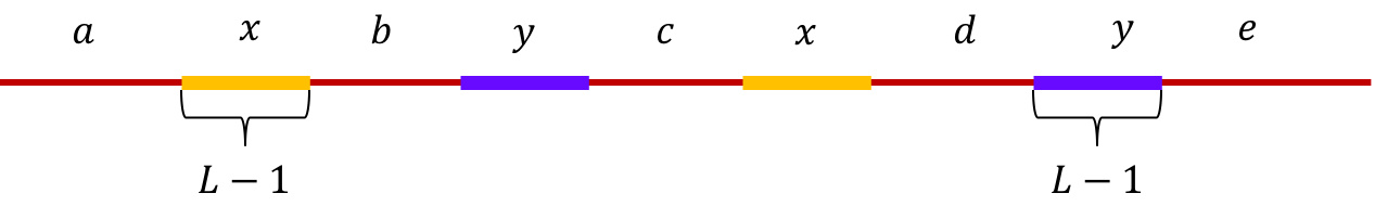
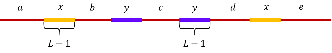
Example 1, Interleaved repeats of length L-1: Let \(x\) and \(y\) be two interleaved
repeats of length L-1 on the genome. Let us assume that the genome has no other
repeat of length L-2 or more.
We show the genome using the shorthand: \(\mathtt{a-x-b-y-c-x-d-y-e}\).
This is illustrated below.
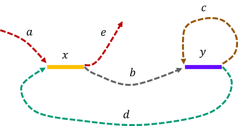
The de Bruijn graph from the L-spectrum of this genome is given by
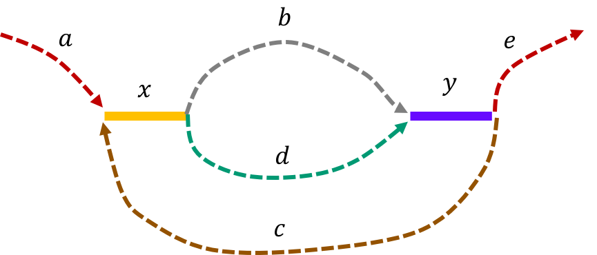
We note that an Eulerian path on the graph would start from \(\mathtt{a - x}\). Then one can either leave \(\mathtt{x}\) through \(\mathtt{b}\) or \(\mathtt{d}\) to get to \(\mathtt{y}\). Any Eulerian path then has to take the path \(\mathtt{c}\) to \(\mathtt{x}\). Then we can take the path not taken from \(\mathtt{x}\) last time to get to \(\mathtt{y}\). This gives us two genomes consistent with the de Bruijn graph : \(\mathtt{a-x-b-y-c-x-d-y-e} \text{ and } \mathtt{a-x-d-y-c-x-b-y-e}\text{.}\)
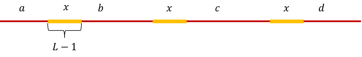
Example 2, Triple repeats of length L-1: Let \(x\) be triple
repeats of length L-1 on the genome. Let us assume that the genome has no other
repeat of length L-2 or more. The genome will be represented using the
shorthand: \(\mathtt{a-x-b-x-c-x-d}\)
This is illustrated below.
The de Bruijn graph from L-spectrum of this genome is given by
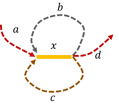
We note that that an Eulerian path on the graph would start from \(\mathtt{a - x}\). Then one can either leave \(\mathtt{x}\) through \(\mathtt{b}\) or \(\mathtt{c}\) to get back to \(\mathtt{x}\). The path then leaves \(\mathtt{x}\) using the other path out to return a third time to \(\mathtt{x}\). Finally, the path leaves \(\mathtt{x}\) through \(\mathtt{d}\). This gives us two genomes consistent with the de Bruijn graph: \(\mathtt{a-x-b-x-c-x-d} \text{ and } \mathtt{a-x-c-x-b-x-d.}\)
In both these examples we have that \(L-1= \ell_{\text{interleaved}}\) , and thus genome can not be assembled from the L-spectrum as stated in the necessary condition of the theorem. Next let us look at examples where the L-spectrum can be used to assemble the genome by the de Bruijn graph algorithm, giving some intuition why the condition is also sufficient.
Example 3, Simple repeat of length L-1: Let \(x\) be simple repeats of length L-1 on the genome. Let us assume that the genome has no other repeat of length L-2 or more. The genome will be represented using the shorthand: \(\mathtt{a-x-b-x-c}.\)
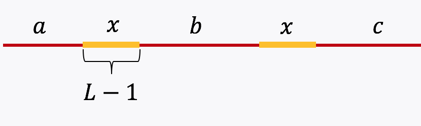
The de Bruijn graph from L-spectrum of this genome is given by
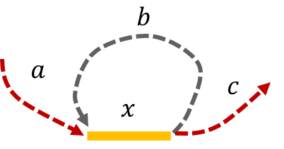
It is easy to see that the only Eulerian path on this de Bruijn graph is the one corresponding to \(\mathtt{a-x-b-x-c}.\) Note that the greedy algorithm may have chosen the path \(\mathtt{a-x--c}.\)
Example 4, Non-interleaved pair of repeats of length L-1: Let \(x\) and \(y\) be two non-interleaved repeats of length L-1 on the genome. Let us assume that the genome has no other repeat of length L-2 or more. We show the genome using the shorthand: \(\mathtt{a-x-b-y-c-y-d-x-e}\).
The de Bruijn graph from L-spectrum of this genome is given by
It is fairly easy to show that \(\mathtt{a-x-b-y-c-y-d-x-e \ \ }\) is the only Eulerian path in the de Bruijn graph.
A practical algorithm based on the de Bruijn graph algorithm
We note that the de Bruijn graph algorithm would work if we had the L-spectrum of a genome and \(L-1 > \ell_{\text{interleaved}}\). However the number of reads of length \(L\) necessary to get the L-spectrum would be astronomical even for modest genome sizes and large read lengths.
To get a more practical version of the de Bruijn graph algorithm, we have to go through a detour. We basically try to get the k-spectrum of a genome from reads of length L where L > k. Abstractly, each read of length L gives us L-k+1 strings of length k (called k-mers). To quantify the number of reads necessary for this to work, given a success probability \((1-\epsilon)\), we must characterize the number of L length reads necessary to get the k-spectrum.
Reads of length L are said to k-cover if there is a read starting in every L-k+1 window of the genome. Note that this means that for every read, there exists a second read with its starting position within L-k+1 positions after the starting position of the first genome. Note that a set of reads k-covering a genome implies that one can recover the k-spectrum of the genome from the reads (Can you see why?).
Consider the following practical algorithm to assemble:
Sample reads enough to get k-coverage.
Run the de Bruijn graph algorithm with the k-spectrum thus obtained.
Here we note that k is a tradeoff parameter. For the algorithm to succeed we need that k - 1 > \(\ell_{interleaved}\), the length of the longest interleaved repeat. Thus a larger k makes assembling more genomes possible; however, larger values of k lead to smaller values of L-k+1. k coverage tells us that we need to get a read starting in every L-k+1 window of the genome, so one would need to sample more reads.
Using similar calculations to those used in the last lecture, we get the following graph describing the number of reads necessary for an algorithm to succeed.
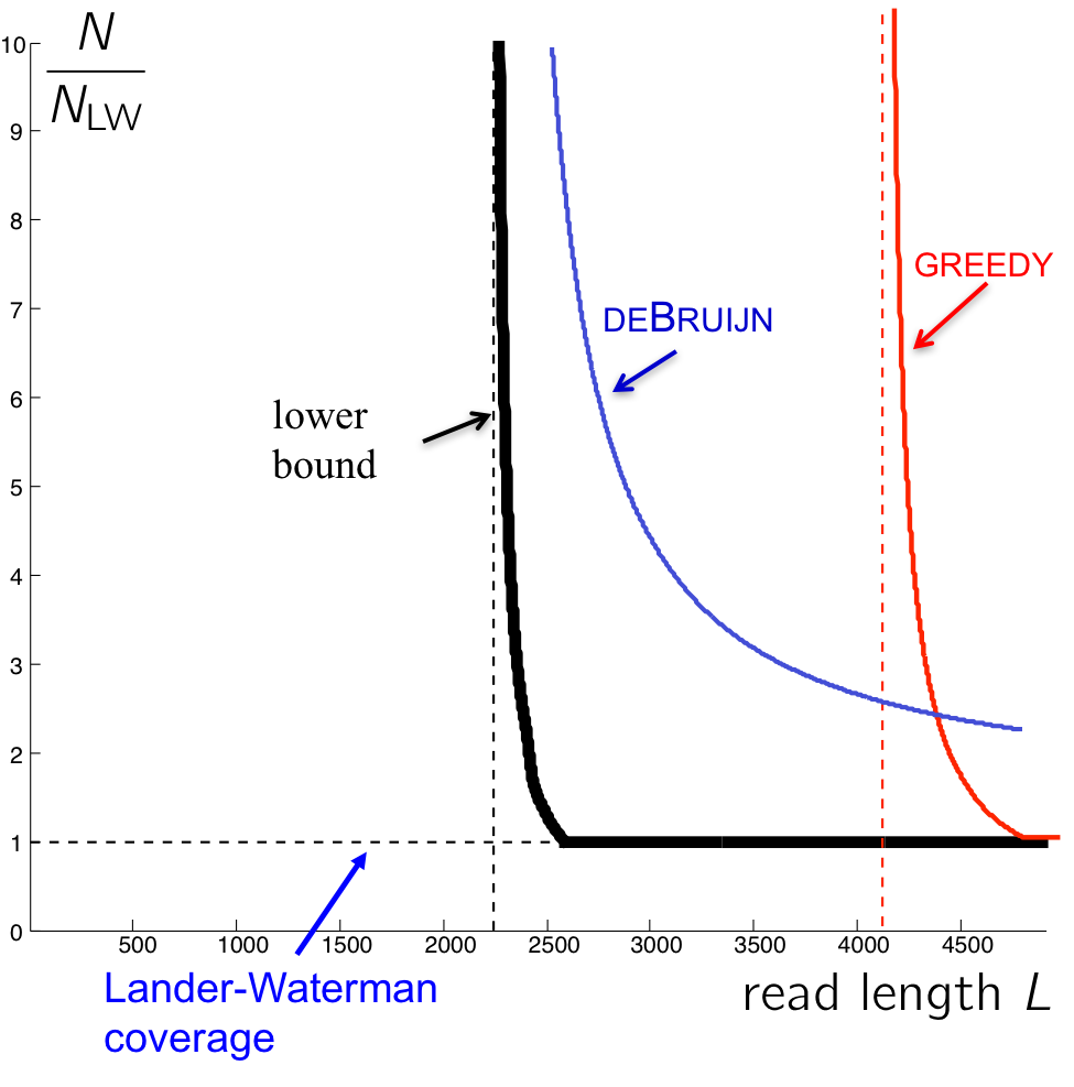
The curve for the de Bruijn algorithm is computed by setting \(k = \ell_{interleaved} + 1\), thus it is the most optimistic performance achievable, since in reality the algorithm does not know \(\ell_{interleaved}\) and has to be more conservative. We note that though the de Bruijn graph algorithm achieves the vertical asymptote, it does need a fairly large number of reads to do so. Although greedy has a worse vertical asymptote, it is better for larger values of L since it requires less reads.
The reason the de Bruijn curve does not match the Bresler-Bresler-Tse’s lower bounds is because it requires every \(\ell_{\text{interleaved}}\)-mer on the genome to be bridged (Note that k-coverage means every k-2 mer in the genome must be bridged. Why?) rather than just having the interleaved repeat bridged. In the next lecture, we will see a tweak of the de Bruijn graph algorithm that tackles this problem to achieve better performance.