Lecture 7: Assembly - Necessary Conditions for Successful Assembly
Lecture 7: Assembly - Necessary Conditions for Successful Assembly
Monday 18 April 2016
Scribed by Vivek Kumar Bagaria and revised by the course staff
Topics
- The greedy algorithm (cont.)
- Interleaved Repeats
- Necessary conditions for genome assembly
- Dense Read Model and the L-spectrum
- de Bruijn Graphs
The greedy algorithm (cont.)
At the end of last lecture, we had proved the following theorem. Recall that a repeat is a subsequence of the genome that appears in multiple places. A repeat is also maximal in the sense that it cannot be extended and still be a repeat.
Theorem. Let a set of reads from a genome fully cover the genome. Moreover, suppose each repeat in the genome is bridged by at least one read. In other words, there exists a read that starts at least one base before a copy of every repeat and ends at least one base after. Then the greedy algorithm is guaranteed to reconstruct the original DNA.
We note that the condition for this algorithm to succeed depends upon a property of the genome that is being inferred (i.e. if its repeats are bridged). Thus a priori given a set of reads, it is not clear if the greedy algorithm will succeed. Despite this, we note that this theorem can be applied in two ways:
- One could run the greedy algorithm on a set of reads. If this returns a sequence, then one can find the set of all repeats in the assembled sequence and check if each one of them is bridged. If that is the case then we have a certificate of the greedy algorithm succeeding in assembling the underlying genome. If there are any unbridged repeats, then whether the greedy algorithm has returned the right genome is unclear.
- We can use the theorem to compute the read lengths and coverage necessary for the greedy algorithm to succeed in known genomes. This can be used as a benchmark on its performance.
Given a known genome \(\mathcal{G}\) of length \(G\), the probability that the greedy algorithm will succeed assembling from \(N\) reads of length \(L\) is the probability that every repeat in \(\mathcal{G}\) is bridged by a read.
To compute this we begin by computing the probability that a repeat of length \(\ell_{\text{repeat}}\) is bridged by a read of length \(L\). We note that this happens if the read starts at a position in the \(L-\ell_{\text{repeat}}-1\) window before either repeat (Note that the bridging condition requires the read to extend at least one base after the repeat, and hence the \(-1\)). We also assume that there exists at least 1 base between the two repeats. Thus,
\[P(\text{A given read of length L bridges a repeat of length } \ell_{\text{repeat}}) = \begin{cases} 0 & \text{if L } < \ell_{\text{repeat}}+2\\ \frac{2(L-\ell_{\text{repeat}}-1)}{G} & \text{otherwise}. \end{cases}\]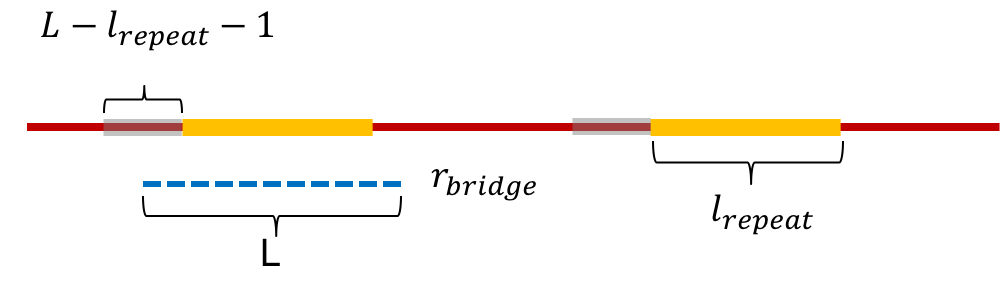
Thus we have that,
\[\begin{align*} P(\text{A repeat of length } \ell_{\text{repeat}} \text{ not bridged by } N \text{ reads of length } L) &= \begin{cases} 1 & \text{if L } < \ell_{\text{repeat}}+2\\ \left(1 - \frac{2(L-\ell_{\text{repeat}}-1)}{G} \right)^N & \text{otherwise}, \end{cases}\\ &\approx \begin{cases} 1 & \text{if L } < \ell_{\text{repeat}}+2\\ \exp\left( -\frac{2N(L-\ell_{\text{repeat}}-1)}{G} \right) & \text{otherwise}. \end{cases} \end{align*}\]Let the genome \(G\) have \(m\) repeats of lengths \(\ell_1, \ell_2, \cdots, \ell_m\). If a repeat appears 5 times, then it is counted 5 times towards \(m\). Further, let us assume that \(\ell_i < L-1\) for \(1 \le i \le m\). After getting \(N\) reads of length \(L\) from the genome,
\[\begin{align*} P(\text{At least one repeat is unbridged}) &\le \sum_{i=1}^{m} P(\text{Repeat } i \text{ is unbridged}),\\ &\approx \sum_{i=1}^{m} \exp\left( -\frac{2N(L-\ell_{i}-1)}{G} \right),\\ &= \exp\left( -\frac{2N(L-1)}{G}\right) \left(\sum_{i=1}^{m} \exp\left( \frac{2\ell_{i}}{G} \right) \right),\\ &= \exp\left( -2c + \frac{2N}{G}\right)\left( \sum_{i=1}^{m} \exp\left( \frac{2\ell_{i}}{G} \right)\right), \end{align*}\]where \(c=\frac{NL}{G}\) is the coverage depth, and the first inequality follows from a union bound. To change the perspective a bit we define,
\[a_{i} = \text{Number of repeats in } \mathcal{G} \text{ of length i, }1 \le i \le L-2.\]This gives us that,
\[\begin{align*} P(\text{At least one repeat is unbridged}) &\le \exp\left( -2c + \frac{2N}{G}\right)\left(\sum_{i=1}^{L-2} a_i \exp\left( \frac{2i}{G} \right)\right). \end{align*}\]We note that to compute this upper bound on probability of failure of greedy algorithm, the number of repeats of a given length, \(a_1,a_2,\cdots, a_{L-2}\) are sufficient statistics (and if there is a repeat of length atleast \(L-1\), greedy fails with probability \(1\)).
Interleaved Repeats
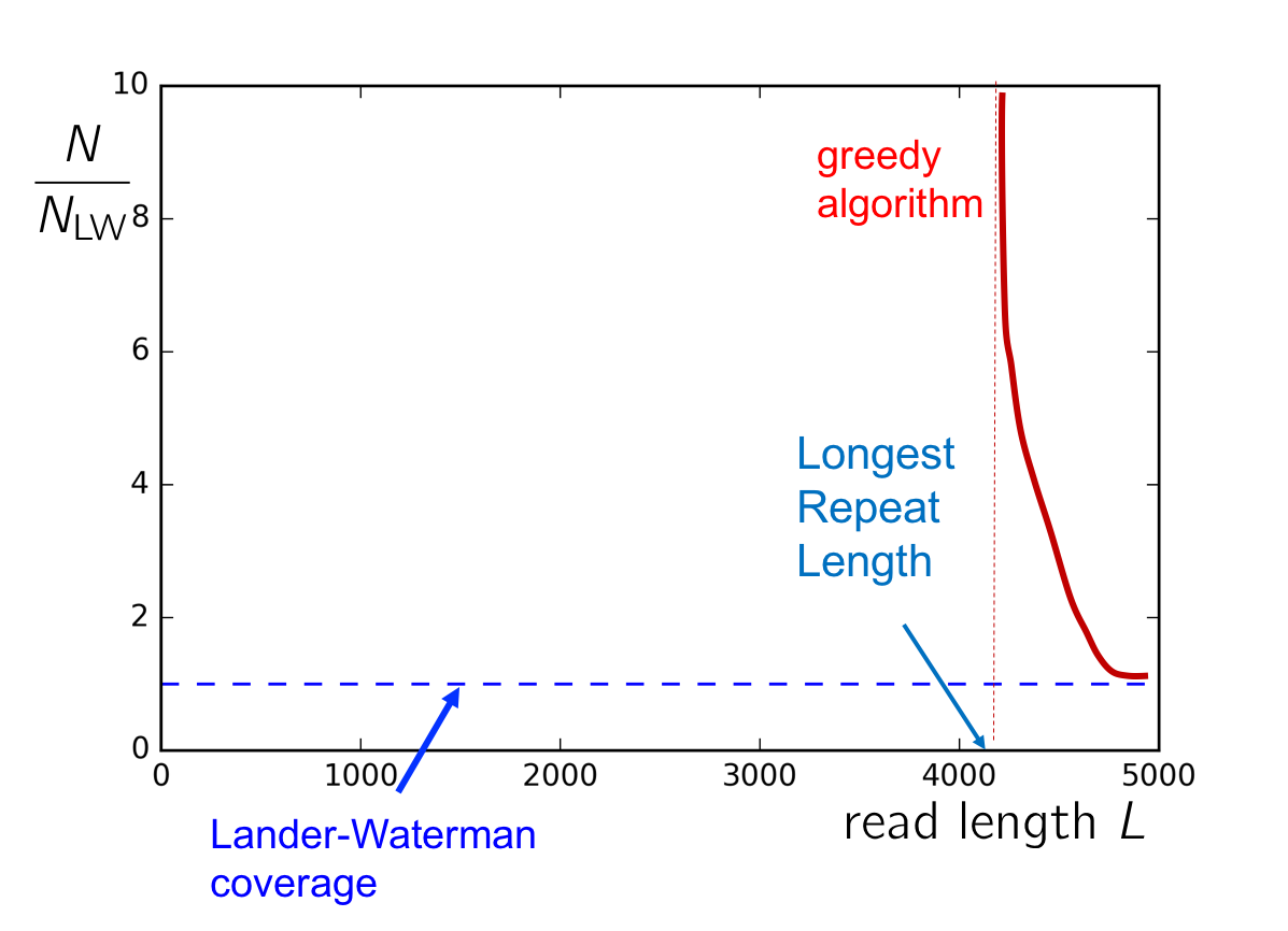
In the last two sections we gave a lower bound on the number of reads necessary for assembly using the Lander-Waterman calculation. We then went through the greedy algorithm and derived the number of reads necessary to achieve a given probability of successful assembly.
This number is shown below for an example genome, Chromosome 19. We note that while the Lander-Waterman calculation gives us a lower-bound independent of the repeat statistics of the genome, the greedy algorithm gives us an achievable scheme that depends upon repeat statistics of the genome. In particular, we note the greedy algorithm fails if the read length is smaller than the length of the longest repeat in the genome. In this section, we derive a genome-dependent lower-bound on both the read length and number of reads required for successful assembly.
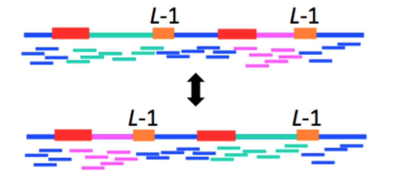
A pair of repeats are said to be interleaved repeats if they appear alternately in the genome. The length of the shorter of two interleaved repeats is called the length of the interleaved repeat. For example, in the figure below, \(r_1\) and \(r_2\) are interleaved repeats, and the length of the interleaved repeat is the length of \(r_2\).
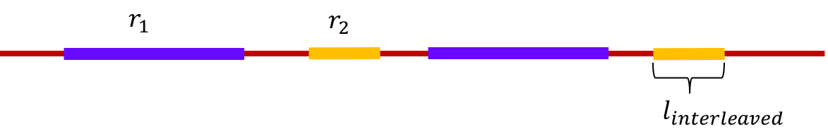
An interleaved repeat is said to be bridged if at least one copy of one of the repeats is bridged.
Triple Repeats
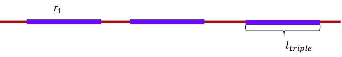
A triple repeat is a repeat that appears thrice in the genome. This is a special case of an interleaved repeat. This is illustrated below.
Necessary conditions for genome assembly
Theorem [Ukkonen 1992; Bresler, Bresler, and Tse 2013]: Assembly of a genome is impossible if any interleaved repeat is not bridged.
As a corollary, we note that this theorem means that the at least one copy of a triple repeat needs to be bridged for assembly of a genome to be feasible.
Proof by picture
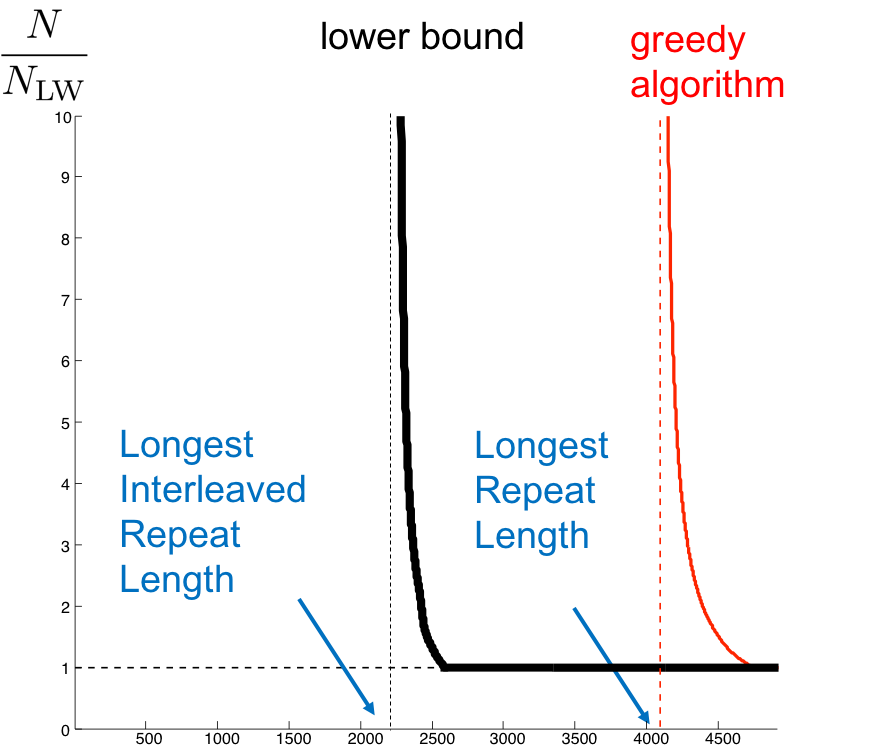
Using calculations almost identical to those used in quantifying the performance of the greedy algorithm, we can derive a curve showing the number of reads necessary for successful assembly in a given genome. This is shown for an example genome below
Dense Read Model and the L-spectrum
To come up with an algorithm that performs better than the greedy algorithm, we first take a detour. We consider an idealized setting called the dense read model. Trying to solve the assembly problem in this setting gives us an algorithm which we can then modify for the shotgun sequencing case.
A dense read model assumes that we have a read starting at every position in the genome. The multi-set of reads thus obtained is called the L-spectrum.
This is illustrated below.
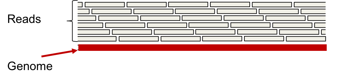
The L-spectrum can be thought of as the set of all unique length-L reads we obtain when we have infinitely many reads from the genome \(\mathcal{G}\) (unique in terms of position).
de Bruijn graphs
In graph theory, the standard de Bruijn graph is the graph obtained by taking all strings over any finite alphabet of length \(\ell\) as vertices,= and adding edges between vertices that have an overlap of \(\ell-1\). In the following, we consider assembly using a slightly modified version of the standard de Bruijn graph from the L-spectrum of a genome.
Given the L-spectrum of a genome, we construct a de Bruijn graph as follows:
-
Add a vertex for each (L-1)-mer in the L-spectrum.
-
Add k-edges between two (L-1)-mers if their overlap has length L-2 and the corresponding L-mer appears k times in the L-spectrum.
An example de Bruijn graph construction is shown below.
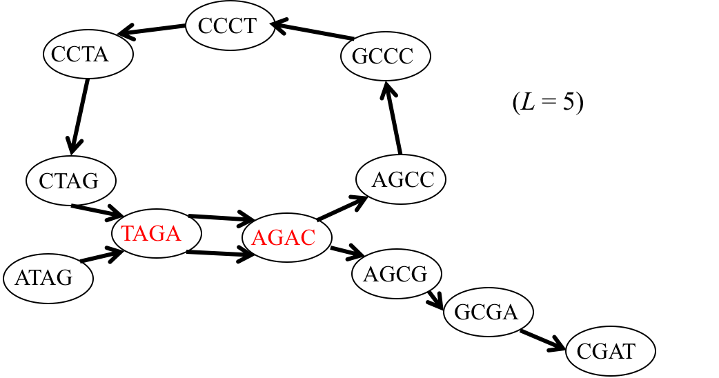
We note that an Eulerian path in the de Bruijn graph corresponds to a sequence consistent with an L-spectrum. Thus if a de Bruijn graph corresponding to the L-spectrum of a genome has a unique Eulerian path, then a genome can be assembled from its L-spectrum.
Theorem [Pevzner 1995]: If L - 1 is strictly greater than the maximum interleaved repeat length of a genome, then the de Bruin graph corresponding to the L-spectrum of the genome has a unique Eulerian path corresponding to the original genome.
This gives us Ukkonen’s lower bound; successful assembly can be achieved as the number of reads become arbitrarily large.