Lecture 5: Assembly - An Introduction
Lecture 5: Assembly - An Introduction
Monday 11 April 2016
Scribed by Mojtaba Tefagh and revised by the course staff
Topics
Reads from a sequencer
We have already gone through a high-level description of the roles of the sequencer and the base caller and how these are achieved in practice. Assuming that these stages are completed successfully, their output would be hundreds of millions to billions of erroneous reads. This information is usually provided to us in the format of a FASTQ file in which \(Q\) stands for the quality score associated to each base
where \(P_e\) is the probability of error which is calculated in the base calling stage and is available alongside the corresponding reads. The next phase in the pipeline is to reconstruct the original genome from this data.
The genome assembly problem
The genome assembly problem simply stated is the following: Given reads coming from a genome can one reconstruct the genome. There are two relevant flavours of this problem. One is the de novo assembly problem which involves reconstructing the genome from just the reads. This is relevant when a previously unsequenced organism is sequenced for the first time. The other is called reference-based assembly, which involves using side information like genomes of individuals of other organisms of the species, whose sequence is known.
There are two major difficulties to genome assembly:
- As mentioned above, errors are ubiquitous in our input data. This can be ameliorated in low error-rate sequencing technologies like Illumina, for which one can restrict their attention to only the high quality reads, and thus wasting a lot of data (for 1% error rates, around one-third of 100 length reads have at least 1 error). However, for simplicity and clarity, we first assume that reads are error free, and examine the assembly problem under that setting.
- By the nature of evolution, there are always a lot of repeats in the genome which make the distinct reads from different far away locations similar. This inherent property of genome makes reads from different places in the genome indistinguishable, which in turn makes it very hard to assemble them.
- Reads are randomly located, which means that there may be some positions in the genome which are thinly covered or not even covered.
In the sequel we will focus mainly on de novo assembly. We will attempt to answer the following questions:
- How many reads do we need to assemble?
We need at least one read that sequences each base of the genome. In other words, we need reads to at least cover the genome Because of the randomness involved in the locations we are sampling from, higher probability of coverage we need, more the samples we need. -
How long reads do we need to assemble the underlying genome unambiguously?
For example, one can not assemble from reads of length 1. So in general we want to get an estimate of the read lengths needed to assemble unambiguously. - How to design efficient assembly algorithms that can operate with minimum number of reads and read length?
Coverage
Let
\[\begin{align*} G &:= \text{Length of the genome},\\ L &:= \text{Read length},\\ N &:= \text{Number of reads}. \end{align*}\]In any case, we would need that \(N > \frac{G}{L}\). If we could pick the positions we could sample, then we could get coverage from these many reads. Note that this is equivalent to,
\[c = \frac{NL}{G}>1.\]Note that \(c\) is the expected number of reads covering a specific position on DNA and called the coverage depth. Furthermore, suppose that reads are sampled uniformly at random and also independent of each other. Under these assumptions, the probability that no read covers location \(i\) can be computed as follows:
\[\Pr(\text{No read covers location }i) = 1-\frac{L}{G}\]Applying this, using the independence of read sampling,
\[\Pr(\text{there exist a location covered by no read})=\left(1-\frac{L}{G}\right)^N=\left(1-\frac{L}{G}\right)^{\frac{G}{L}\cdot\frac{LN}{G}}\approx e^{-\frac{LN}{G}}=e^{-c}\]Define the random variable \(X\) to be the number of positions not covered by any reads. By the linearity of expectation, the above line implies that:
\[\begin{align*} E[X]=Ge^{-c} \\ \Rightarrow \Pr(X\geq 1) \leq \frac{E[X]}{1}=Ge^{-c} \\ \Rightarrow \Pr(X=0)\geq 1-Ge^{-c} \end{align*}\]where the second step holds because of Markov inequality. Therefore, if one wants to guarantee the coverage with a probability of failure at most \(\epsilon\), it is enough to consider the following \(N\):
\[\epsilon=Ge^{-c}\Rightarrow c=\ln\frac{G}{\epsilon}\Rightarrow N=\frac{G}{L}\ln\frac{G}{\epsilon}\]As an example, if the genome of interest is about one billion base pairs long, and the probability of failure is set to \(1\%\), then we need at least \(25\)X coverage depth. \((G=10^9;\epsilon=0.01\Rightarrow c=25.328)\)
Greedy Algorithm
We note that the above coverage itself does not say if a genome can be assembled. For example, we could get length read \(1\) and cover the genome but not be able to assemble the genome. Thus it is clear that, the read length is related to if we can assemble a genome or not. To get a handle on this relationship, we start with a simple algorithm to assemble, and understand its limitations. These limitations will give us some insights, into barriers for assembly.
Consider the following greedy assembler:
while (# reads > 1)
{
    Search among all pairs of reads and find the two with the largest overlap
    merge these two so that the number of reads is reduced by one.
    Exit if no overlap found.
}
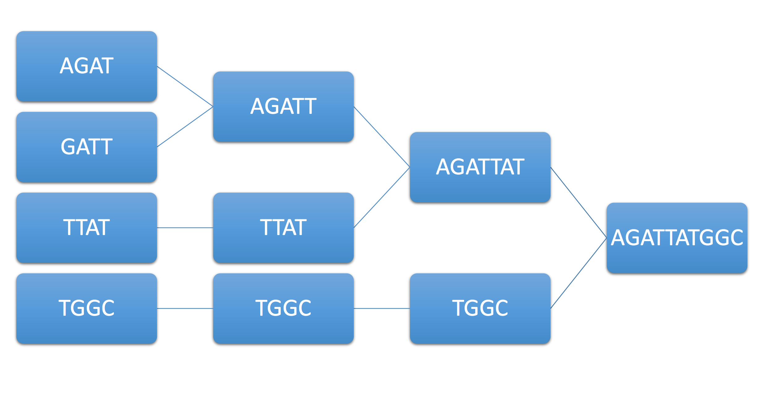
As an example of how this works, consider the example genome \(AGATTATGGC\) and its associated reads \(AGAT,GATT,TTAT,TGGC.\) Then the above algorithm assembles them as follows:
As another example, consider the example genome \(ATGGTATGGC\) and its associated reads \(ATGG,TGGT,TATG,TGGC.\) Then the greedy algorithm assembles them in the following wrong way:
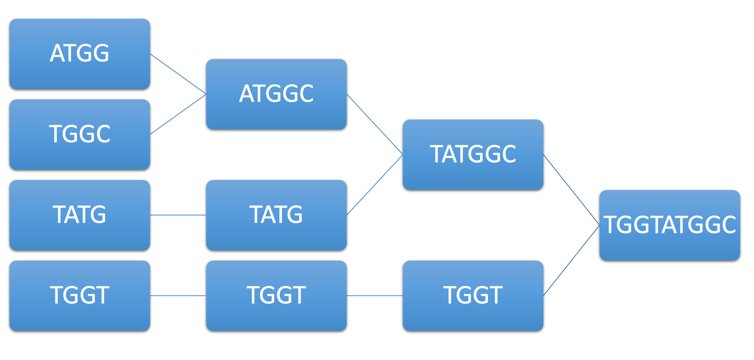
As you can see, we cannot always guarantee that the output of the greedy algorithm is the original DNA. The following theorem gives the necessary and sufficient conditions for the correct assembly:
Theorem. Let a set of reads from a genome fully cover the genome. Moreover, let each repeat in the genome be bridged by at least one read, that is there exists a read that starts at least one base before every repeat, and ends at least one base after. Then the above greedy algorithm is guaranteed to reconstruct the original DNA in the absence of noise.
Proof: We first prove that by contradiction that we never merge any two reads incorrectly.
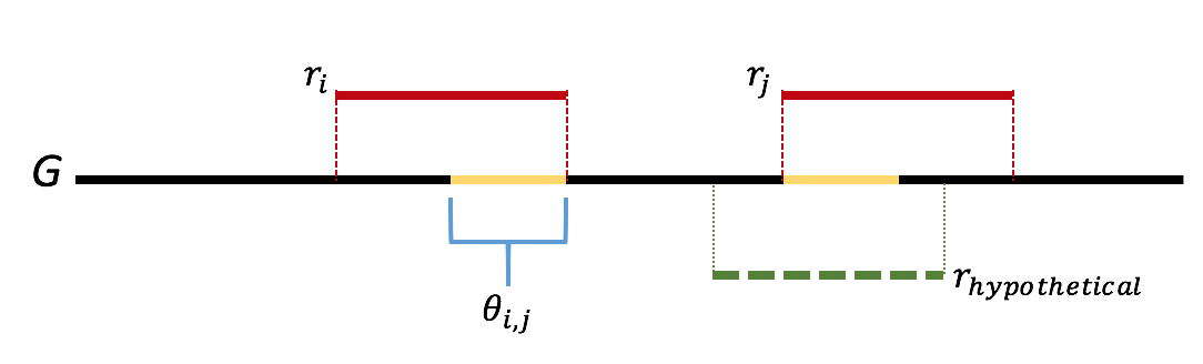
Let \(\ell\) be the first step where we we incorrectly merge two reads. Let \(r_i\) and \(r_j\) be the two reads incorrectly merged. Let \(\theta_{i,j}\) be the overlap between reads \(r_i\) and \(r_j\). We further note that the greedy nature of the algorithm means that all overlaps of length greater than that of \(\theta_{i,j}\) are already merged. We note that this means that the sequence \(\theta_{i,j}\) appears twice in the genome. Further we note that if either appearance of \(\theta_{i,j}\) was bridged, then one of \(r_i\) or \(r_j\) would have had a overlap longer than the length of \(\theta_{i,j}\), which we would have merged first. This gives us that \(\theta_{i,j}\) is not bridged, which is contradiction. This gives us that there is never an incorrect merge in the algorithm. This argument is illustrated in the figure below.
Because the genome is assumed to be covered, we are left with a single sequence when the algorithm terminates. As we have made no mistakes in our merging, this is our underlying sequence, proving the result.
- The two illustrations of the greedy algorithm are by to Mojtaba Tefagh.