Lecture 3: Base Calling for Second-generation sequencing

Lecture 3: Base Calling for Second-generation sequencing

Monday 4 April 2016

Scribed by Alborz Bejnood and revised by the course staff

Topics

In the previous lecture, we learned about the evolution of first and second generation sequencing efforts. In this lecture, we examine the base calling step in the process of sequencing DNA: the inference of individual bases from a series of light intensity signals.

1. Base calling for Illumina sequencing
2. Error sources
3. Modeling the error source
   • The error model
   • Inference on the model
     • Zero-forcing
     • Minimum mean square error based estimation
     • Maximum likelihood estimation
     • Epilogue to the estimation story

Base calling for Illumina sequencing

We begin with a review of the sequencing by synthesis approach to sequencing. We start with DNA and fragment it into many shorter sequences (resulting in a number of fragments on the order of 100 million to 1 billion). Then on glass plates, there are a number of dots onto which these DNA fragments will stick, with the material on the plate complementary to the basis on those dots. Not every dot will have a such a fragment, but a good fraction of them will, allowing us to move towards sequencing. We recall that the solution contains two entities: ddNTP (free-flowing) and DNA polymerase (binds the ddNTP). In addition, there is the enzyme that reverses termination in the washing cycles.

We note that the above is a simplified version of base calling. In reality, the fluorescent signal from a single template is too weak to be detected. Hence, first the template is converted into many clones using a technique called polymerase chain reaction (PCR) (which also won its discoverer Kary Mullis a Nobel prize). Before synthesis, each strand is cloned using PCR and each dot corresponds to 1000 clones per strand. Ideally one would want all copies of fragments in a dot to be synchronized going forward. Because of chemical and mechanical imperfections, some strands are lagging behind and others are leading forward in the same dot leading to a lot of “noise” in a dot.

Error sources for Illumina sequencing

The main source of errors is the asynchronicity of the various molecules in a dot.

In a cycle there are molecules where two ddNTPs are attached (due to the first one being attached being a dNTP rather than a ddNTP). This is shown in pane 3 in cycle 1 in the figure below. Here the molecule bound to a dGTP rather than a ddGTP. Thus the synthesis was not terminated, and the molecule bound to a ddATP as well. This led to it emitting light corresponding to A rather than G, leading to an inconsistency with a molecule where this defect may not have occurred. This results to the strand leading.

Another error would occur if termination is not reversed in the washing cycle. In the figure below, this is shown in pane 2 in cycle 3. Here the termination of G is not reversed. Thus this molecule emits light corresponding to G rather than light corresponding to A. This leads to an inconsistency in the corresponding output signal (compared to a molecule where this has not occured). These strands are said to be lagging.

An illustration showing errors in illumina sequencing, showing different molecules in a dot.

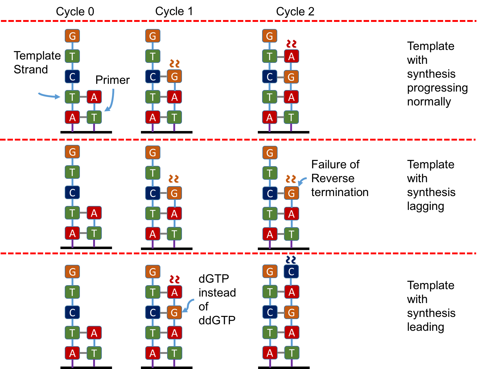
Both leading and lagging errors are called phasing errors.

Modeling the error sources and doing inference

The error model

We probabilistically model the problem as follows. Let \(L\) be the length of the molecule being sequenced. Let the original sequence be \(\mathbf{s}=s(1),s(2),\cdots,s(L).\) Let us define sequences \(\mathbf{s}^{(A)},\mathbf{s}^{(C)}, \mathbf{s}^{(G)}, \mathbf{s}^{(T)}\), as

Let \(\mathbf{y}^{(A)}, \mathbf{y}^{(C)}, \mathbf{y}^{(G)}, \mathbf{y}^{(T)}\) be the intensities of the colours corresponding to A, C, G, and T respectively. We note that we make \(L\) measurements in total (one measurement per cycle), and hence each one of \(\mathbf{y}^{(A)}, \mathbf{y}^{(C)}, \mathbf{y}^{(G)}, \mathbf{y}^{(T)}\) is an \(L\) length vector. We define

Further we define

Now we model the relationship between \(\mathbf{y}^{(A)}\) and \(\mathbf{s}^{(A)}\). Here we observe that at time \(i\), the intensity is given by

where \(n_i\) is noise that we model as zero mean Gaussians \(\mathcal{N}(0,\sigma^2)\), independent across cycles, and \(b\) is the total intensity expected if all molecules had the same colour emitted. We note that the signal observed in cycle \(j\) depends not only on \(s^{(A)}(j)\) but upon all other values of \(\mathbf{s}^{(A)}\). In statistical signal processing, this is called inter-symbol interference.

In matrix notation, this problem reduces to

Inference on the model

Zero-forcing

The most obvious inference rule would be

where \(\mathbb{I}\) is the usual indicator function, that is

In signal processing literature, this is referred to as Zero-forcing.

We note that

where \(\mathbf{n}_{ZF} \sim \mathcal{N}(0, \sigma^2 Q^{-1}(Q^{-1})^{T})\) . That is, the noise across co-ordinates are not independent. This formulation is suboptimal if \(Q\) is an ill-conditioned matrix, i.e. if the largest singular value of Q is much larger than the smallest singular value of Q. To see this at a high level, let \(\sigma_{\max}^2, \sigma_{\min}^2\) be the largest and the smallest singular values of \(Q\). Next note that the noise variance of \(n_{ZF}\) in the dimension corresponding to the largest singular value of \(Q\) is \(\frac{\sigma^2}{\sigma_{\max}^2}\), which is much smaller than the \(\frac{\sigma^2}{\sigma_{\min}^2}\), the noise variance of \(n_{ZF}\) in the dimension corresponding to the largest singular value of \(Q\). The probability of making an error is determined to a first order by the latter which can be quite bad.

Minimum mean square error based estimation

Another popular estimator is the Minimum mean square error (MMSE) estimator. This is basically derived by picking \(\hat{\mathbf{s}^{(A)}}\) such that \(\mathbb{E}[(\hat{\mathbf{s}^{(A)}}-\mathbf{s}^{(A)})^2]\) is minimised. In the standard setting when the support of \(\mathbf{s}^{(A)}\) is not restricted to be \(\{0,1\}\), this leads to \(\hat{\mathbf{s}^{(A)}}= \frac{1}{b} Q^T(QQ^T+\sigma^2 I)^{-1}\mathbf{y}^{(A)}\).

The MMSE-based estimator used in this setting is

Maximum likelihood estimation

The maximum-likelihood estimator for this case would involve running the Viterbi algorithm. This basically involves solving

The time complexity of the Viterbi algorithm is exponential in the recursion depth (which in here is the maximum |i-j| if there is non-zero probability of seeing light from base j at time i). In this setting, this is \(O(2^{L})\). A work-around this is to approximate each column of \(Q\) so that it is non-zero only in a \(w\) width band. This gives the run time of the maximum-likelihood to be \(O(2^{w}L)\). This is quite managable for \(w \le 10\).

Epilogue to the estimation story

One could estimate \(\mathbf{y}^{(A)}, \mathbf{y}^{(C)}, \mathbf{y}^{(G)}, \mathbf{y}^{(T)}\) separately and then combine these estimates; however, this is clearly suboptimal. A better estimation procedure is to write these as a linear estimation problem and use the straight-forward generalisations of the techniques discussed above. The linear system would be

Illumina initially used an algorithm called Bustard, which essentially did zero-forcing on this system. Then, algorithm BayesCall was proposed, which essentially does the MMSE based estimation on this system. BayesCall is currently the most popular algorithm. The authors of BayesCall also proposed another algorithm called NaiveBayesCall which approximates the Viterbi algorithm on the above system.