Lecture 16: RNA-seq - Hard EM and De Novo Transcriptome Assembly
Lecture 16: RNA-seq - Hard EM and De Novo Transcriptome Assembly
Monday, May 23, 2016
Scribed by the course staff
Topics
Analysis of Hard EM
Last time, we talked the EM algorithm and its particular application to the problem of RNA-seq quantification. We discussed two versions of EM: the hard EM and the soft EM. In the context of quantification, if a read is multiply mapped to several different transcripts, then we split the read so that each transcript gets a fraction of a count. We showed that the iterative EM algorithm always converges to the maximum likelihood solution. EM always converges to a local optimum because every iteration always increases the likelihood function. In particular, the likelihood function for the RNA-seq quantification problem is concave, and therefore EM will converge to the global optimum.
For hard EM, the count of the read is mapped to only transcript \(i\) where
\[i^* = \text{argmax}_{i} \rho_i\]Consider the example from last lecture. We have \(t_1\) consisting of exons A and B and \(t_2\) consisting of exons B and C. The ground truth is \(\rho_1 = 1.0\) and \(\rho_2 = 0.0\). We have 20 reads that come from \(t_1\), 10 that maps to exon A and 10 that maps to exon B. We will need to break ties randomly; i.e. each read that maps to exon B is assigned to \(t_1\) and \(t_2\) with equal probability. Notice that in this case if we break ties randomly, at some point more reads will be assigned to \(t_1\).
Now let’s consider the case where we have \(\rho_1 = 0.9\) and \(\rho_2 = 0.1\). We obtain the read mapping shown in the figure below (the figure enforces our assumption that the transcripts, and in this case exons, are equal).
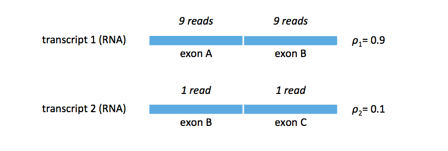
We can walk through the hard EM algorithm. If ties are broken in favor of \(t_1\), then
\[\begin{align} \rho_1^{(1)} & = \frac{19}{20} = 0.95 \\ \rho_2^{(1)} & = \frac{1}{20} = 0.05. \end{align}\]On the other hand, if ties are broekkn in favor of \(t_2\)< then
\[\begin{align} \rho_1^{(1)} & = \frac{9}{20} = 0.45 \\ \rho_2^{(1)} & = \frac{11}{20} = 0.55. \end{align}\]The algorithm breaks (i.e. we are not guaranteed to converge to the correct solution). The take-home message here is that while both the soft and hard EM algorithms seem intuitive, only one actually works. While EM was invented in 1977, it was only applied to the quantification problem in 2010 by Trapnell et al. in their tool Cufflinks.
In practice, most transcripts have different lengths. In the homework, you will consider what happens when transcripts have different lengths and when minor errors exist.
De Novo Transcriptome Assembly
We now look at more complicated problem: the situation where we do not know the transcripts. While for humans there exists a well-curated set of transcripts, this may not be true for other (in fact, most) organisms. Additionally, even in human cancer the set of transcripts may be very different from the known set of human transcripts.
In this problem, we are again given the reads. We want to reconstruct the set of transcripts and estimate their abundances. We will again refer to the transcripts as \(t_1, \dots, t_K\) and tie abundances as \(\rho_1, \dots, \rho_K\). We know longer know the \(t_i\). One approach would be to pretend that all sequences up to a length are possible transcripts, and we can perform quantification on this large transcriptome. Of course, if \(\ell = 1000\), our transcriptome will consist of \(4^{1000}\) potential transcripts (and abundances to estimate).
The actual transcriptome, however, is much smaller and on the order of 10,000s of transcripts. By running vanilla EM on all \(4^{1000}\) candidates does not exploit this fact is, among other reasons, is computationally inefficient.
Assembly approach
There are two ways to view this problem: one from the assembly end and one from the quantification end. We can leverage some of our knowledge from assembly to facilitate recovery of an unknown transcriptome.
Recall that the de novo assembly problem involves reconstructing an unknown sequence from a given set of reads. The de novo transcriptome assembly problem is similar, only we have potentially 10,000s of sequences rather than 1, and the set of reads we obtain are from all of the sequences. For the single-sequence case, we drew the plot shown in the figure below in lecture 5, describing the critical number of reads needed for assembly.
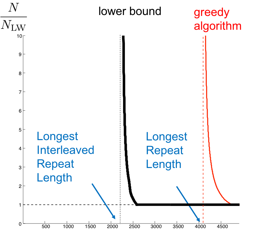
Can we use the algorithms we’ve previously discussed for the transcriptome recovery problem? Unlike for the genome case, different transcripts appear in different abundances. To determine the above curve for this problem is quite difficult. We will instead explore on how we can get a handle on \(L_{crit}\) for this harder problem. Recall that \(L_{crit}\) is the longest interleaved repeat on the genome. The fact that we need a minimum read length assemble is because there is an inherent repeat structure to the sequence, which produces ambiguous reads and causes confusion.
Going back to our first example in this lecture, we notice that there are repeats in the transcriptome (e.g. exon B is repeated across the two transcripts). With the repeat sequences spanning different transcripts, we expect \(L_{crit}\) to somehow capture this. Note that there may exist repeats within a transcript, but typically this does not happen. The majority of repeats happen across transcripts, and this is the case we will focus on.
Recall that for the single-sequence case, we assumed that the coverage is so dense that we had a read at every position of the genome (\(L\)-coverage). This assumption allowed us to recover \(L_{crit}\). For the unknown transcriptome case, the \(L\)-spectrum will be given by all reads of length \(L\) at every starting position on the transcript. We still have a problem; ambiguous reads across shared exons.
For the transcriptome recovery case, the count (the number of occurrences) of a read is the sum of the number of transcripts on which the read appears. The \(L\)-spectrum is the set of all length \(L\)-subsequences of all transcripts together with these counts. We will attempt to reconstruct the transcripts together with the abundances using this information.
Consider the example transcriptome in the figure below. Does this transcriptome have a unique \(L\)-spectrum? i.e. Does there exist another transcriptome with the same \(L\)-spectrum?
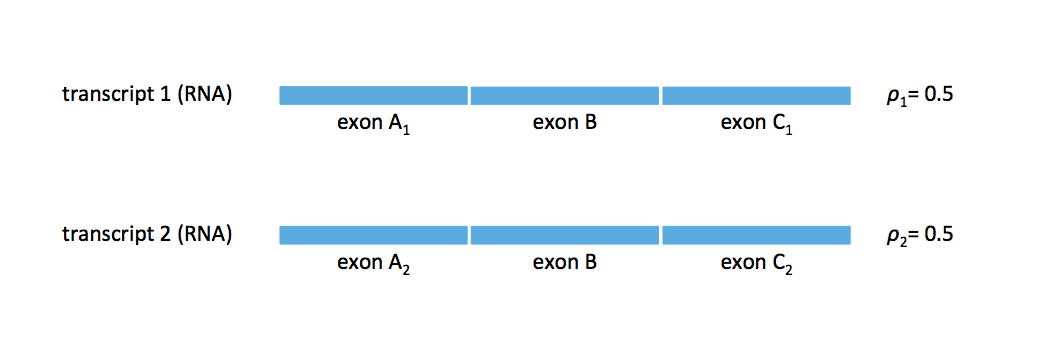
Notice that if we have another two-transcript transcriptome where exons A\(_1\) and A\(_2\) are switched, then we cannot distinguish before the two transcripts. We need a read that bridges exon B in order to resolve this ambiguity. Therefore we have ambiguity if the read length is shorter than the length of exon B.
If we make the assumption that reads are sampled uniformly from a transcript, then would expect reads to be uniformly spread across each transcript. Therefore we can leverage the counts of reads to rule one transcriptome more likely than another, as shown in the figure below.
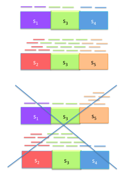
We can think of each exon (A\(_1\), A\(_2\), B, C\(_1\), C\(_2\)) as a node with edges describing the abundances, and we can solve the problem by casting it as a flow problem. The graph below shows the graph corresponding to the transcriptome above with two potential flows. There are 3-flow situations with \(\rho_1 \neq \rho_2\). We will consider these in the next lecture.
IMAGE OF NODE GRAPH