Lecture 14: Wrapping up Haplotype Assembly and Introduction to RNA-seq

Lecture 14: Wrapping up Haplotype Assembly and Introduction to RNA-seq

Monday 16 May 2016

Scribed by the course staff

Topics

In this lecture, we will wrap up the community recovery perspective on the haplotype assembly problem by examining another way to relax the NP-hard formulation introduced last lecture. We will then transition into computational problems related to a new topic: RNA-seq.

1. Phasing problem
   • SDP relaxation
   • Comparing the spectral and SDP methods
2. RNA-seq
   • A counting problem

Phasing problem

Last time, we introduced an interpretation of the phasing problem. Recall the data matrix \(Y\). Recall that

We formulated the phasing problem as a maximum likelihood problem:

We argued last lecture that it’s actually NP-hard in general. Our strategy was to relax the problem somehow to something more tractable. Last time, we relaxed the domain of \(x_i\) to all real numbers while constraining \(\|x\|_2 = n\). If the measurements (reads) are randomly and uniformly spread throughout the genome, then this relaxation can be shown to get optimal recovery. We performed a sanity check by verifying \(E[Y]\) is a rank-1 matrix with the principal eigenvector equal to the true underlying \(\mathbf{x}\). Under this assumption, we have that

where \(\mathbf{x}\) is the ground truth.

In practice, we usually get reads that link together SNPs that are close to each other. With this, we have that the expected data matrix \(\mathbb{E}[Y]\) is not necessarily a rank 1 matrix. For example, if we had 3 SNPs which are all +1 and n observations (which are the SNPs separated by 1 or 2), then the expected data matrix is,

which has rank 2.

We see that the spectral method does not work even with \(\mathbb{E}[Y]\) in this case, and thus the spectral method has a lack of robustness property.

SDP relaxation

Here we will introduce another type of relaxation: the semidefinite programming (SDP) relaxation. We first exploit some clever properties from linear algebra to reformulate the optimization problem.

We used the fact that \(\text{tr}(AB) = \text{tr}(BA)\), assuming that \(AB\) and \(BA\) are both valid matrix multiplications. \(\text{tr}(X)\) is the trace of matrix \(X\) or the sum of \(X\)’s diagonal entries. We also defined \(\mathbf{X} = \mathbf{x} \mathbf{x}^T\). Notice that \(\mathbf{X}\) is rank 1, symmetric, and each entry is also in \(\{+1,-1\}\) (because \(x_i \in \{+1,-1\}\)). Also, all diagonal entries of \(\mathbf{X}\) are equal to 1, i.e. \(\mathbf{X}_{ii} = 1 \ \forall \ i\). The optimization problem now becomes

This problem is still NP-hard due to the rank constraint. Because \(X\) is rank 1 and symmetric and its eigenvalues are \(n\) and 0, we can relax the rank constraint:

where \(\mathbf{X} \succeq 0\) indicates that \(\mathbf{X}\) must be positive semidefinite (i.e. \(\mathbf{v}^T \mathbf{X} \mathbf{v} \geq 0 \ \forall \ \mathbf{v}\)). A positive semidefinite matrix must have non-negative eigenvalues. The problem is now convex, since \(\text{tr}(\mathbf{Y}\mathbf{X})\) and \(\mathbf{X}_{ii} = 1\) are linear constraints and the set of \(\mathbf{X}\) that satisfies \(\mathbf{X} \succeq 0\) is a convex set. It turns out that under the uniformly spread out model, we can show that if there is enough information, then the SDP relaxation gives us a reasonable solution.

Comparing the spectral and SDP methods

We will now compare the two methods we’ve introduced for efficiently solving the community recovery problem. (We note that neither method has been shown to work for the haplotype phasing problem as is.)

In terms of efficiency, the spectral method wins. Computing the principal eigenvector of a matrix can be done using the power method where we multiply a random vector with the same matrix over and over again. We can solve a problem with n = 100000 in less than a minute on a laptop. SDP is much slower and on the order of \(O(n^3)\).

In terms of robustness, the SDP relaxation can be shown to have good performance for some settings of “benevolent-adversaries” (see Moitra, Perry, and Wein 2015 for details. A surprising result proved there is that “benevolent-adversaries” make the learning task strictly harder.)

RNA-seq

So far, all the material covered in this course has revolved around working with data from DNA. From high school biology, you might recall something called the central dogma of molecular biology, an illustrative (but very oversimplified) diagram of how genetic information flows within an organism.

The central dogma of molecular biology.

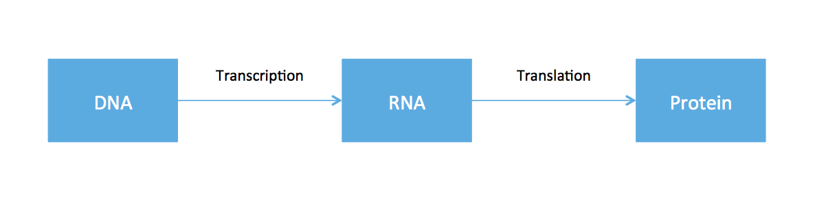
The cell functions by using DNA as the blue-print to to create proteins. Ribonucleic acid (RNA) is produced as an intermediate product. While every cell in the body has roughly the same DNA, cells in different tissues clearly have varying functions. This is because different cells express different RNA. Therefore if one is interested in the dynamics of different cell types, one should somehow measure RNA. While DNA is static, RNA expression can be different depending on time, tissue, and environmental factors.

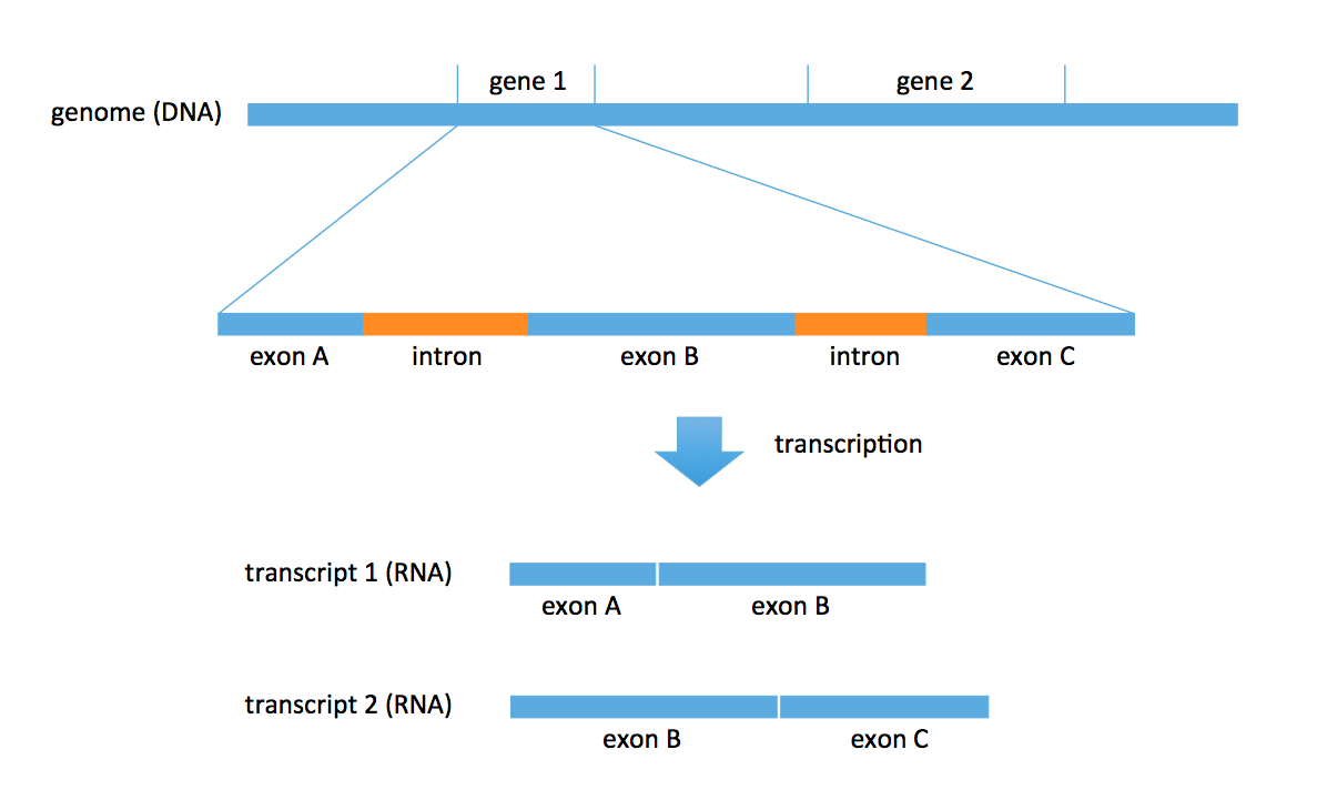
DNA consists of two parts: coding and noncoding. The coding part includes objects called genes. There are roughly 27000 annotated genes in humans, occupying about 1% of the entire genome. A lot of biology revolves around these genes; for example, RNA is transcribed from these genes. Each gene also consists of multiple parts: exons and introns. In the transcription problem, we take a subset of these exons to form an RNA transcript. We could obtain multiple transcripts from the same gene. In the figure below, we obtain 2 distinct transcripts from gene 1, a transcript consisting of exons A and B, and another transcript consisting of exons B and C.

Transcription of genes into RNA transcripts.

There are known genes for which there are 1000s of different types of transcripts (for example, neurexin) produced by the gene. Most genes produce 5-10 versions of transcripts (or isomers). Transcripts are typically 1000-20000 bp long.

For a given cell, some genes may be expressed and others may not be expressed. The genes that get expressed may have 1 or more isoforms, and each isoform may be expressed in different abundances. Within a cell, we may see tens of thousand of transcripts from the union of all the genes.
A biologist would be interested in identifying these transcripts. Estimating gene expression is the problem of figuring out which transcripts are expressed and at what abundance.

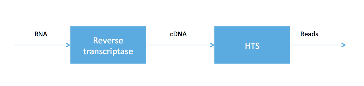
As we said at the beginning of the course, high-throughput sequencing (HTS) is very useful because HTS technologies can be applied to measure other molecules. In RNA-seq, we sample a tissue and, after some chemistry, obtain a soup of RNA transcripts. Biologists have been able to convert the RNA to a special type of DNA (called cDNA) using an enzyme called reverse transcriptase, and we can feed the DNA into our high-throughput sequencer. The pipeline is summarized in the figure below.

The RNA-seq pipeline.

RNA-seq was developed in Mortazavi et. al., 2008. We will focus on computational problems related to getting short reads (100 bp Illumina reads, for example) for RNA-seq.

A counting problem

Let’s say we have two transcripts that appear in different abundances. We get reads randomly from the two transcripts but proportionally to their abundances. We want to infer which transcripts are present and what their abundances are. There are multiple flavours of the problem (listed in order of increasing difficulty):

1. Transcripts are known but the abundances are not.
2. Neither transcripts nor abundances are known. The genome is known.
3. Neither transcripts nor abundances are known. The genome is also not known.

We may encounter the first case if we are working with a popular organism such as a human or mouse. In this case, there exists a curated set of transcripts called the transcriptome. Additionally, different tissues will have different abundances, and this information is the subject of differential analysis. We may encounter the second case if we are looking at an organism whose transcriptome is not known, or cancerous tissue (where the transcriptome is changed by change in genome, but all transcripts seen are reasonably long sequences from the original genome stitched together).

We will start with the first formulation. The computational problem here is a counting problem: we want to count how many reads came from each transcript. Mapping reads to transcripts can be done using various alignment algorithms, which we’ve discussed in previous lectures. Notice that there is an intrinsic ambiguity here: in some cases, one does not know where a read comes from. For example, consider transcripts 1 and 2 in the figure above. If we obtain a read that aligns to exon B, then we cannot tell which transcript it came from. This is an inference problem. Most ambiguities result from different transcripts sharing exons. For simplicity, we currently will not worry about the different lengths of transcripts (this is easy to account for later).

In summary, we have two types of reads: uniquely mapped and multi-mapped. The processing of Mortazavi et. al., 2008 just used the uniquely mapped reads to do inference.

Let \(t_i, \dots, t_k\) be \(k\) transcripts and \(\rho = (\rho_1, \dots, \rho_k)^T\) be the abundances of the transcripts. We obtain N reads \(R_1, \dots, R_N\), and we want to estimate \(\rho\). Let \(N_k\) be the number of reads that map uniquely to transcript \(k\) and \(N = \sum_k N_k\) be the total number of unique reads. Let

In the above example, if we had a third transcript that consists of only exon A, then no part of its sequence would be unique. Therefore the approach of Mortazavi et. al., 2008 will not see any reads from this transcript and we will always obtain an abundance of 0.

Alternatively, we can assign partial counts. In the above example with two transcripts, if we obtain a read that aligns to exon B, we can give half a count to each transcript. This also has its own issues. For example, if the underlying truth is \(\rho_1 = 1\) and \(\rho_2 = 0\), then only transcript 1 is expressed. This scheme will not give us an estimate of 0 for transcript 2. We will address this problem in the next lecture.