Lecture 13: Haplotype Assembly - Community Detection
Lecture 13: Haplotype Assembly - Community Detection
Wednesday 11 May 2016
Scribed by Christian Choe and revised by the course staff
Topics
In the last lecture we introduced the haplotype assembly problem. By casting the problem as a convolutional coding problem, we can use Viterbi decoding to arrive at a solution. This approach suffers from an exponential runtime in terms of the number of SNPs between mate-pairs. In this lecture, we will take a different approach based on the community recovery problem.
Community recovery problem
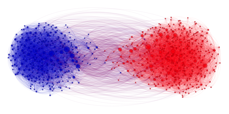
In the community recovery problem, we are given a graph with a bunch of nodes, and each node belongs to one of multiple clusters as shown in the figure below. The recovery problem is to recover the clusters (colors) based on the edge information between nodes. This problem is commonly seen in social networks where nodes can be blog posts, for example, and we want to identify which posts are from Republicans and which are from Democrats. The edges describe how the posts link to one another.
Haplotype assembly
When sequencing a haploid organism, we obtain a set of heterozygous SNPs such as the one shown in the figure below. ‘0’ and ‘1’ represent the different SNPs.
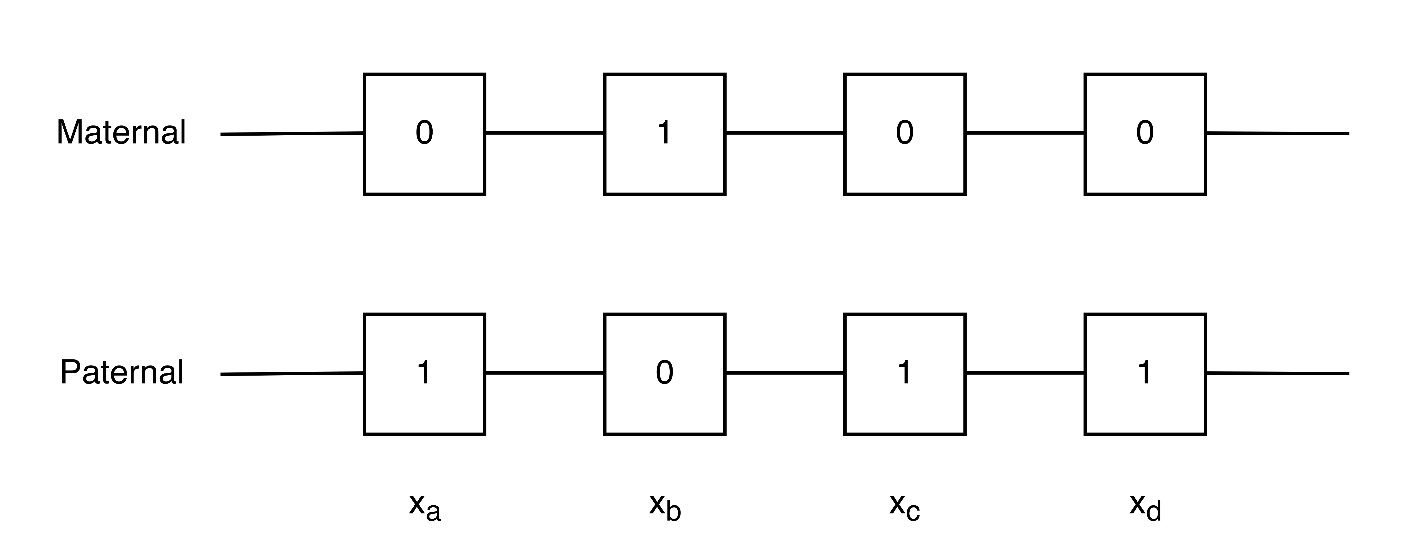
If we represented this as a graph, we would have four nodes corresponding to the 4 heterozygous SNP locations. We can also define two communities \(A\) and \(B\) for our graph:
\[A = \begin{bmatrix} 0 \\ 1 \end{bmatrix} \ \ \ \ \ \ \ B = \begin{bmatrix} 1 \\ 0 \end{bmatrix}\]Nodes \(a, c,\) and \(d\) belong to community \(A\), and node \(b\) belongs to community \(B\). In practice, we may have 100,000 nodes with half in each cluster. Notice that recovering the communities is equivalent to solving the haplotype phasing problem. The partition will give us all the information except for 1 bit: which SNPs correspond to the maternal chromosome.
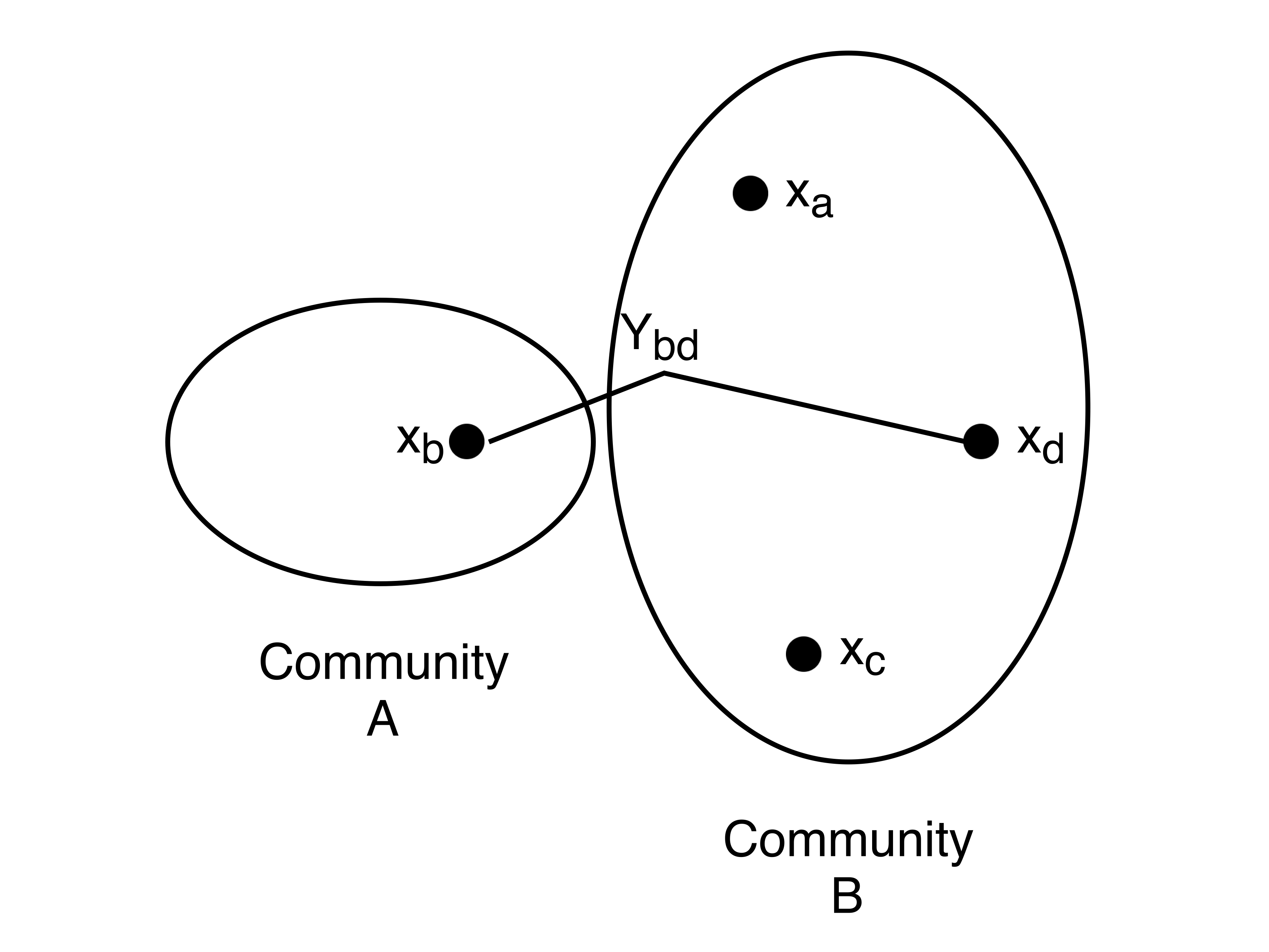
We will let \(x_i\) denote the class of node \(i\) and \(x_i \in \{-1,+1\}\). Let \(Y_{ij}\) represent the edge data between nodes \(i\) and \(j\) where \(Y_{ij} = 1\) if \(x_i == x_j\) and -1 otherwise. We will set \(Y_{ij} = 0\) if there is no linking reads between node i and node j. If there is no noise, then \(Y = 1\) corresponds to an edge where the two nodes are in the same community and vice versa. \(Y = -1\) would indicate the two nodes being in different communities. The figure below illustrates the notation introduced so far.
When working with real read data, we can think of each measurement (mate-pair read) as a noisy edge on the graph telling us if two nodes are linked. We introduce a random variable \(Z_{ij}\) to represent the noise in each edge. We assume that all \(Z_{ij}\) are i.i.d. In summary,
\[\begin{align} x_i & \in\ \{-1, 1 \} \\ Z_{ij} & = \left\{ \begin{array}[cc]\\ 1 & \text{w.p. } 1- \epsilon\\ -1 & \text{w.p. } \epsilon \end{array}\right. \\ Y_{ij} & = x_i x_j Z_{ij} \end{align}\]\(Y_{ij}\) essentially tells us if two nodes are in the same community with an \(\epsilon\) probability of error. Exploiting vector notation, we further define:
\[\mathbf{x} = \begin{bmatrix} x_1 \\ \vdots \\ x_n \end{bmatrix} \in \mathbb{R}^n \\ \mathbf{Y} = \left[ Y_{ij} \right] \in \mathbb{R}^{n\times n}\]Maximum likelihood
To solve the community recovery problem, we will use maximum likelihood to infer the \(x_i\)’s’:
\[\begin{align} \hat{\mathbf{x}} & = \text{argmax}_{\mathbf{x}} P\left(\mathbf{Y}|\mathbf{x} \right) \\ & = \text{argmax}_{\mathbf{x}} \prod_{i,j \in E} P\left(Y_{ij} | x_ix_j \right) \\ \end{align} \\ P\left(Y_{ij} | x_ix_j \right) = \left\{ \begin{array}[cc]\\ 1 - \epsilon & \text{if } Y_{ij} = x_ix_j \\ \epsilon & \text{if } Y_{ij} \neq x_ix_j\epsilon \end{array}\right.\]where \(E\) indicates the set of edges in the observed data. This can be further simplified by using the log likelihood:
\[\hat{\mathbf{x}} = \text{argmax}_{\mathbf{x}} \sum_{i,j \in E} \log\left(P\left(Y_{ij}|x_ix_j \right)\right)\]where each log term can be expressed as
\[\begin{align} \log\left(P\left(Y_{ij}|x_ix_j \right)\right) & = \left\{ \begin{array}[cc]\\ \log\left(1 - \epsilon\right) & \text{if } Y_{ij} = x_ix_j \\ \log\left(\epsilon\right) & \text{if } Y_{ij} \neq x_ix_j\epsilon \end{array}\right.\\ & = Y_{ij}x_ix_j\left(\frac{\log(1-\epsilon) - log(\epsilon)}{2}\right) + \frac{\log(1-\epsilon) + \log(\epsilon)}{2} \end{align}\]Since \(\epsilon\) is a constant, we can further simplify the ML decoder to
\[\begin{align} \hat{\mathbf{x}} & = \text{argmax}_{\mathbf{x}} \sum_{i,j \in E} Y_{ij}x_ix_j\\ & = \text{argmax}_{\mathbf{x}} \sum_{i,j} Y_{ij}x_ix_j\\ & = \text{argmax}_{\mathbf{x}} \ \mathbf{x}^T \mathbf{Y} \mathbf{x} \end{align}\]Notice that we threw in the edges that are not in the observed set of edges. We can set \(Y_{ij} = 0\) for these cases. Ultimately, we want to compute the maximization using this quadratic form. Brute force maximization of this is quite bad because the number of possible \(\mathbf{x}\)’s is \(O(2^n)\).
Intuitively, when two nodes are in the same community (\(x_i x_j =1\)) and there is no error (\(Z_{ij} = 1\)), \(Y_{ij}\) is positive, giving us a positive contribution to our maximization objective. We do not want negative terms. We can decompose the sum in objective into:
\[\begin{align} \sum_{i,j} Y_{ij}x_ix_j & = (\text{# of in-cluster $+1$ edges}) \\ & + (\text{# of cross-cluster $-1$ edges}) \\ & - (\text{# of in-cluster $-1$ edges}) \\ & - (\text{# of cross-cluster $+1$ edges}) \\ \end{align}\]This is a combinatorial optimization problem. Suppose we are solving a simpler problem where we only have \(-1\) edges. Then the objective becomes
\[\begin{align} \sum_{i,j} Y_{ij}x_ix_j & = (\text{# of cross-cluster $-1$ edges}) - (\text{# of in-cluster $-1$ edges}) \\ & = |E| - (\text{# of cross-edges}) \\ & = 2 - (\text{# of cross-edges}) - |E| \end{align}\]While the number of edges is fixed, the number of cross edges depends on the clustering. Therefore the problem becomes: find a partition of the graph that maximizes the number of cross edges. This is the max cut problem, which is NP hard. If we approach the problem from a general approach, it’s NP hard. We will need to exploit some further structure in the problem.
Spectral method
In order to solve this NP hard combinatorial optimization problem, we can use the spectral method to arrive at an approximate solution. We relax the problem by allowing each \(x_i\) to be real. We will also constrain \(\|\mathbf{x}\|_2 = n\). We can bound the optimization problem as follows:
\[\begin{align} & \max_{\mathbf{x}} \sum_{i,j} Y_{ij}x_ix_j \\ = & \max_{x_i, x_j \in \{\pm1\}} \mathbf{x^TYx}\\ \le & \max_{\mathbf{x},||\mathbf{x}||_2 = n} \mathbf{x^TYx} \\ \le & \lambda_{max}n \end{align}\]Because \(Y\) is a symmetric matrix, its eigenvalues are real and positive. We simply set \(\mathbf{x}\) to equal the eigenvector corresponding to the largest eigenvalue of \(\mathbf{Y}\). By taking the sign of each entry in \(\mathbf{x}\), we get an approximate solution to our original problem (where \(x_i \in \{-1,+1\}\)) with a reasonable \(\mathbf{x}\). This approach is called the spectral method because we pick \(\mathbf{x}\) according to the spectrum of \(\mathbf{Y}\).
Correctness of spectral method
Because we relaxed the original problem, we need to exhibit some evidence that this approach is good. Consider the following random graph: for every pair of points, we draw an edge between them with probability \(p\). Note that Y is a random matrix because the location of the measurements are random and the errors are random. We want to first check what happens when \(\mathbf{Y}\) is replaced by its expected value. Intuitively, if this method does not work when \(\mathbf{Y}\) is deterministic at the mean, then there’s not much hope of this method working in general.
\[\begin{align} \bar{Y_{ij}} & = E[Y_{ij}] \\ & = (1 - p)\dot\ 0 + p[x_ix_j(1-\epsilon) - x_ix_j\epsilon] \\ & = p(1-2\epsilon)x_ix_j \end{align}\]Therefore
\[\mathbf{\bar{Y}} = p(1-2\epsilon)\mathbf{xx^T}\]\(\mathbf{\bar{Y}}\) is a rank 1 matrix, and applying the spectral method on this matrix will give us exactly \(\mathbf{x}\), our ground truth. The hope is that while \(\mathbf{Y}\) in actuality is random, statistically it’s close to its mean \(\mathbf{\bar{Y}}\). This shows that using the spectral method, we can expect to get a reasonable answer.
The solution obtained for \(\mathbf{\hat{x}}\) using the spectral method will be correct in a large number of entries. We can clean up the entries a bit by considering the neighbors of each node. We set each node to the majority community amongst its neighbors. Since most of the nodes are correct, this clean-up step improves our solution.
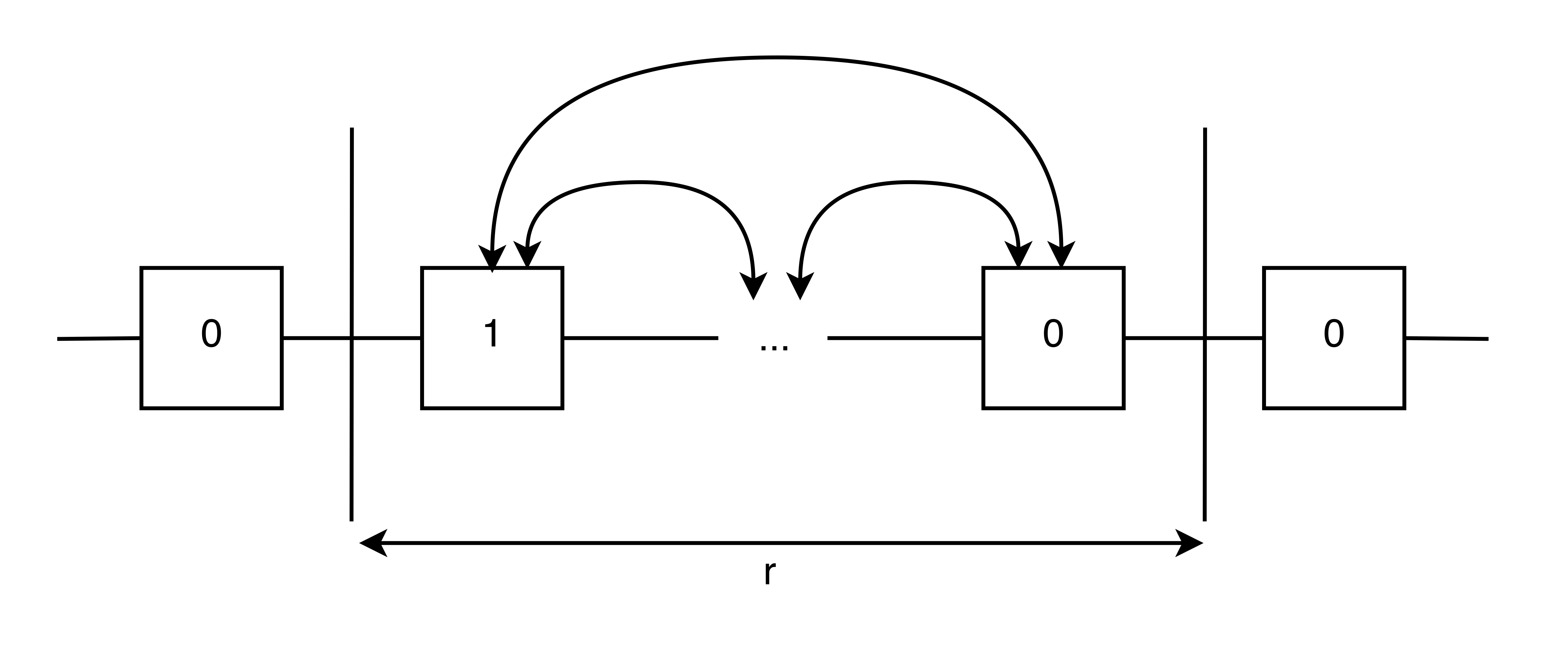
Simplifying the haploid phasing problem
When dealing with real heterozygous SNPs, the linking information will be constrained to ranges of ~100 kbp (e.g. 10x technologies) while the chromosomes they reside on are each ~100 Mbp. Since the links are localized, unlike a random graph, we can section the chromosome into segments of length \(r\) and analyze each segment as shown in the figure below. For small values of \(r\) we can use Viterbi decoding, but for large values we can use the spectral method.