Lecture 12 : Haplotype Assembly - Introduction and Convolutional Codes
Lecture 12 : Haplotype Assembly - Introduction and Convolutional Codes
Monday 25 April 2016
Scribed by Chayakorn Pongsiri and revised by the course staff
SNP calling
Single Nucleotide Polymorphisms (SNPs) are mutations that occur over evolution. A simplistic view of these would be to think of them as around 100,000 positions where variation occurs in the human genome.
SNP calling is a technique that is used to identify SNPs in the sample genome. The main computational approach taken here is given reads from a genome, we first map the reads to various positions on the genome using alignment methods discussed in the last lecture. Some reads map into locations with no variation with respect to the reference.
At a high level, the pipeline can be seen as follows:
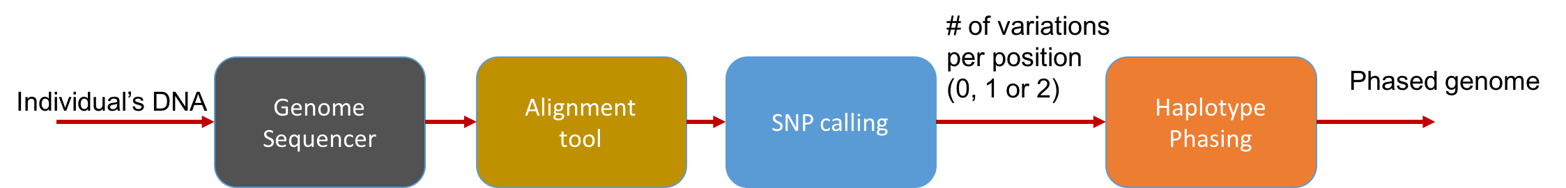
The main statistical problem is to be able to distinguish errors in reads from truly different SNPs in the underlying genome. In practice, we usually have very high coverage; every position in the genome is covered by many reads. Thus we can run a simple statistical test to see if a read disagreeing with the reference is due to errors or due to the individual’s genome actually being different.
SNP calling in diploid organisms
If an organism had only one copy of every chromosome, the SNP calling problem would reduce to just taking the majority of the base of reads aligned to every position. Humans, however, are diploid. They have two copies of every chromosome: one maternal and the other paternal.
During sequencing, we fragment the DNA material, so the sequencer cannot distinguish between the paternal and maternal DNA. When we map these reads to the locations, we do not have as clean a picture. We represent variation in each position as a 1 and no variation as a 0. In each position, we have 4 possibilities:
- 00 (no variation)
- 11 (both copies are different from the reference)
- 10 or 01 (one of the copies is the reference and the other is the variation)
We note that we assume here that there is only one variant at each position. This is a reasonable approximation to reality.
Positions with 00 and 11 are called homozygous positions. Positions with 10 or 01 are called heterozygous positions. We note that the reference genome is neither the paternal nor the maternal genome but the genome of an un-related human (or more precisely the mixture of genomes of a few individuals). An individual’s haplotype is the set of variations in that individual’s chromosomes. We note that as any two human haplotypes are 99.9% similar, the mapping problem can be solved quite easily.
After mapping the reads, we gain information about the likelihood of four above possibilities. For SNP calling, we can measure (estimate) the number of variations at each position: 0, 1, or 2. Note that we cannot tell between the two heterozygous cases (01 vs 10). Distinguishing these two is important because many diseases are multiallelic. That is, multiple positions determine a disease. Also the diseases depend upon the proteins produced in an individual. This depends upon the SNPs being present on the same chromosome rather than being present on different chromosomes.
Haplotype Assembly
Haplotype phasing is the problem of inferring information about an individual’s haplotype. To solve this problem, there are many methods.
First, we focus on a class of methods focused on getting better data (rather than better statistical methods). Let’s say we have two variants, SNP1 and SNP2. The distance between the two are on the order of \(\approx\) 1000 bp (i.e. they’re pretty far apart). To do haplotype phasing, one needs some information that allows us to connect the two SNPs so that one can infer which variants lie on the same chromosome. If you do not have a single read that spans the two positions, then you don’t have any information about the connection between the two SNPs.
Illumina reads are typically 100-200bp long and are therefore too short; however, there does exist multiple technologies that provide this long-range information. We discuss two of these:
-
Mate-pair reads - With a special library preparation step, one can get pairs of reads that we know come from the same chromosome but are far apart. They can be ~1000 bp apart, and we know the distribution of the separation.
-
Read clouds - Pioneered by 10x Genomics, this relatively new library preparation technique uses barcodes to label reads and is designed such that reads with the same barcode come from the same chromosome. The set of reads with the same barcode is called a read cloud. Each read cloud consists of a few hundred reads that are from a length 50k-100k segment of the genome.
For both of these technologies, the separation between linked reads is a random variable, but one can compute it by aligning the reads to a reference.
In practice, the main software used for haplotype assembly are HapCompass and HapCut. HapCut poses haplotype assembly as a max-cut problem and solves it using heuristics. HapCompass on the other hand constructs a graph where each node is a SNP and each edge indicates that two SNP values are seen in the same read. HapCompass then solves the haplotype assembly problem by finding max-weight spanning trees on the graph. For read clouds, a 10x Genomics’s loupe software visualizes read clouds from NA12878, a human genome used frequently as a reference in computational experiments.
The Computational Problem
Here we consider a simplified version of the haplotype assembly problem. We assume we have the locations of the heterozygous positions in the genome, and we only consider reads linking these positions.

The above figure shows two chromosomes with heterozygote SNPs; we want to identify which variations occurred on the same chromosome. Let \(L_i\) = parity between \(i^{\text{th}}\) and \((i+1)^{\text{th}}\) SNP. For example, in the above figure \(L_1 = 1, L_2 = 1, \text{ and }L_3 = 0.\)
The observed parities obtained between the two SNPs covered by the reads are given by \(Y_A = 1, Y_B = 1, \text{ and } Y_C = 1.\) Because the observations are noisy, one can model each SNP observation as the true parity being flipped with some probability \(\epsilon\) independent of all other SNP observations. This leads to the following model:
\(Y_A = L_2 \oplus Z_A\)
\(Y_B = L_1 \oplus Z_B\)
\(Y_C = L_2 \oplus L_3 \oplus Z_C,\)
where \(Z_A, Z_B, Z_C \sim \text{Bernoulli}(\epsilon(1-\epsilon)) \ \ \\) model the noise in the observed parities.
Our goal is to infer the sequence of \(L_i\), allowing us to identify which variations occurred on the same chromosome. Note that we still cannot tell which variations are on the maternal chromosome and which are on the paternal chromosome.
Convolutional Code and Viterbi Algorithm
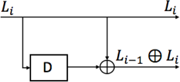
The transfromation from \(L\)’s to \(Y\)’s can be viewed as a convolutional code and the maximum-likelihood decoder is called the Viterbi algorithm.
The runtime of the Viterbi algorithm is linear in the number of SNPs in the genome (around 100,000 in human genome) and proportional to \(2^{\text{mate-pair separation range}}\). The fact that the runtime is exponentially increasing with the mate-pair separation range can be a problem when the range is long. Convolutional codes with constraint lengths (mate-pair separation range) in the tens are routinely decoded in communication using various schemes that trim the state-space.
- Figure 2 here is due to Chayakorn Pongsiri.