Lecture 17: Multiple Testing

Lecture 17: Multiple Testing

Tuesday 6 March 2018

scribed by Andre Cornman and edited by the course staff

Topics

1. Multiple testing
2. Benjamini-Hochberg test
3. Justifying the BH test

Multiple testing

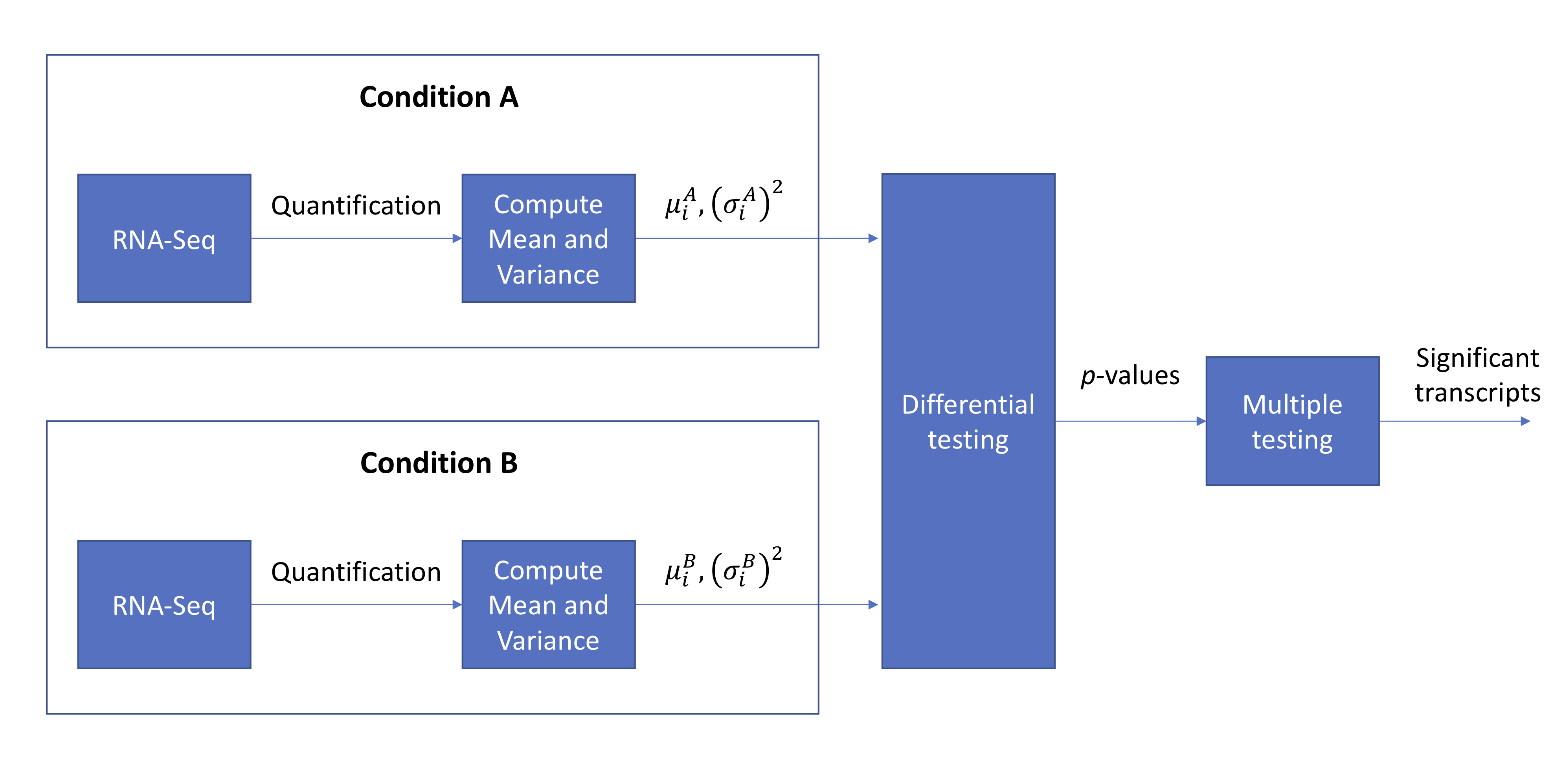
For today’s lecture, we will continue from where we left off at the end of lecture 15. We will go back to talking about bulk RNA-Seq. Recall that this whole procedure can be summarized using the following block diagram:

The statistical testing framework for RNA-Seq.

Last time, we discussed the concept of a \(p\)-value where we let \(P_i\) represent the \(p\)-value for the \(i\)th transcript. We have two important facts about \(p\)-values:

1. A \(p\)-value is a random variable
2. Under the null hypothesis, a \(p\)-value has uniform distribution

We discussed two methods for tackling the multiple testing problem to determine which of the \(m\) tests are significant. Let \(V\) represent the number of false discoveries out of the \(m\) tests:

1. Control FWER (Bonferroni procedure): The family-wise error rate FWER is defined as \(Pr( V > 0)\). To control the FWER at 5% (i.e. \(FWER \leq 0.005\) ), we simply change our rejection threshold from 0.05 to 0.05/\(m\). This approach is rather conservative, however. Perhaps we are willing to allow a few false discoveries if we can make several true discoveries.

2. Control FDR (Benjamini-Hochberg procedure): The false detection rate is defined as \(E\left[\frac{V}{\max(R, 1)} \right]\) where \(R\) represents the number of discoveries. We will discuss a procedure for controlling the FDR in detail below.

Benjamini-Hochberg test

Consider a list of \(p\)-values obtained from a large set of hypothesis tests (e.g. one for each transcript): \(P_1, \dots, P_m\). The Benjamini-Hochberg test was created in 1995 and consists of the following two steps:

1. Sort the \(p\)-values in ascending order to obtain \(P_{(1)} \leq P_{(2)} \leq \dots \leq P_{(m)}\)

2. Plot the sorted \(p\)-values and draw a line with slope \(\alpha/m\). We will reject the null hypothesis for all points before the first crossing of the line of the sorted \(p\)-values from the right

Benjamini-Hochberg procedure figure borrowed from the PH525x series notes.

Intuitively, if we decrease \(\alpha\), the slope of the line decreases, resulting in less \(p\)-values lying under the \(\alpha/m\) curve and therefore less rejections. This makes sense since we expect fewer rejections with a more stringent \(\alpha\).

For the Bonferroni procedure, we consider the hypotheses \(H_1, \dots, H_m\). Importantly, the Bonferroni procedure compares each of the \(m\) \(p\)-values independently to a fixed threshold \(\alpha/m\). For the Benjamini-Hochberg procedure, the decision we make on a test \(H_i\) depends both on \(P_i\) and the other \(p\)-values (captured by the sorting step).

Example

Consider the following set of \(p\)-values obtained from a differential expression test: 0.02, 0.03, 0.035, 0.006, 0.055, 0.047, 0.01, 0.04, 0.015, 0.025.

1. Under the Bonferroni procedure with \(\alpha = 0.05\), we make discoveries on none of the tests.
2. Under the BH procedure with \(\alpha = 0.05\), the first \(p\)-value after sorting that crosses the \(\alpha/m\) line is 0.04. Therefore we make discoveries on the 1st, 2nd, 3rd, 4th, 7th, 8th, 9th, and 10th tests.

Justifying the BH test

The BH-test, while straightforward, seems rather arbitrary at first glance. We will attempt to justify why the BH procedure is indeed valid and controls FDR at \(\alpha\). For simplicity, we start with just one test. We know that under the null \(H_0\), \(P \sim U[0, 1]\) (i.e. the \(p\)-value has a uniform distribution). Under the alternate \(H_1\), then \(P \sim f_1\). The false discovery rate captures the fraction of times the null is actually true despite being rejected:

where \(F_1\) represents the CDF under the alternate, and \(F\) represents the mixture of the null and alternative distributions. To control FDR to be \(\alpha\), set \(\theta\) such that

where we have one equation and one unknown. Taking a step back, recall that Fisher was interested in

Compare this to the probability expression we started with and note that they are not the same! In Fisher’s case, we can just see \(\theta = \alpha\), which is how he came up his rejection procedure. Importantly, to solve this equation, we do not need knowledge of \(F_1\). For our probability of interest, however, we need both \(F_1\) and \(\pi_0\). Therefore we cannot control the FDR in the case of a single testing problem without making strong assumptions on what the alternative looks like.

For the multiple testing scenario, let’s assume that \(P_1 \sim U[0, 1]\) under the null, and \(P_1 \sim f_1\) under the alternate. With, say, \(m = 20000\) tests, we can now solve the above equation because we have 20000 observations drawn from \(F(\theta)\), the mixture distribution. We note that

has a CDF on the right-hand side and a line with slope \(\pi_0/\alpha\) on the left-hand side.

Justifying the decision boundary for the BH procedure.

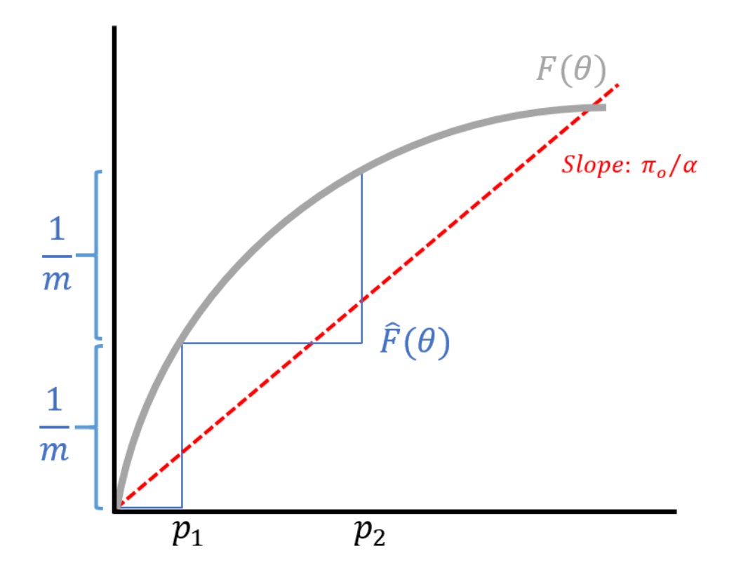
While we do not have \(F\), we have enough samples to compute an empirical approximation of \(F\). Note that for the empirical approximation, the height of each step is \(1/m\). The width of the first step is exactly the smallest \(p\)-value. Intuitively, the sorting step of the BH procedure is captured by computing the approximate CDF.

We flip the two axes and stretch the (new) horizontal axis by \(m\), resulting in a line with slope \(\alpha/(\pi_0 m)\). How do we handle the \(\pi_0\)? We can replace \(\pi_0\) by 1, resulting in a more conservative threshold. Since the less conservative threshold already controlled FDR at rate \(\alpha\), increasing the stringency will still be valid. This final form is now the BH test we introduced in the beginning of the lecture.