Lecture 15: Differential Analysis and Multiple Testing
Lecture 15: Differential Analysis and Multiple Testing
Tuesday 27 February 2018
scribed by Michelle Drews and edited by the course staff
Topics
Introduction
Prior to this lecture, we have worked out the details of an RNAseq experiment from tissue to transcript abundance. Our samples of interest are lysed, the RNA is extracted and purified, then converted to cDNA and run through High Throughput Sequencing, which gives us a set of reads. We then take the reads, and using the EM quantification discussed in the previous lectures, we are able to get transcript abundance.
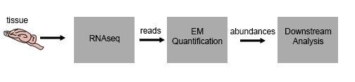
However, this data is somewhat useless on its own – we’d like to draw conclusions
about real biology from these abundances – which generally involves
comparing sequencing data from two different populations/treatments/etc.
However, we need to be careful about how we do this, because given the large
number of transcripts in a given data-set, the likelihood of accepting a
false conclusion becomes large if we use the traditional statistics for single
hypothesis testing multiple times in a row. This problem is generally referred
to as the
Multiple Testing problem,
and is not sequencing specific – in fact, it is relevant to many areas of
bio-statistics, especially in the era of big data.
Differential analysis
In a typical RNAseq experiment in the wild, scientists will have 2
conditions they would like to compare. For this example let’s pretend you’re
Aashish Manglik, and you’ve discovered a groundbreaking new
painkiller.
You want to see how your painkiller changes gene expression, so you do RNAseq
on cells before your treatment, and cells after your treatment – and you want
to know what is the difference between A and B. The type of analysis you are
going to do is a Differential Expression Analysis.
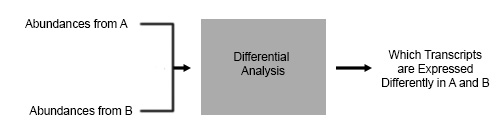
There are many software programs available that do this kind of analysis, such as DESeq and DESeq2 which are R based. The output that we would like to get from our program is a quantification of which transcripts are expressed differently in A and B in the above figure.
However, “which transcripts are expressed differently” is not a very
mathematically precise statement – so let’s expand on this further.
We’re interested in things that aren’t just different – we’re interested in
things that are statistically different, using some statistical method.
Let’s start working through the analysis, and we’ll illustrate this
example as we go.
We start the analysis with transcript counts for each condition from our
EM algorithm (Salmon or Kallisto or RSEM or Cufflinks, or others).
In practice, this can be a count of the number of reads per transcript
or number of reads mapped to a particular gene (remember: a gene can have
multiple transcripts), or an abundance metric for each transcript.
All these data are roughly equivalent with each other, since counts
are just scaled abundances and the math is the same for transcripts
and genes – there’s just more transcripts than genes.
Suppose the output of this is the following (say A being a control and B being a treatment group).
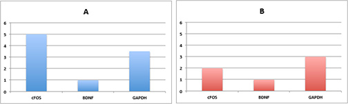
Just looking at this data, with our patented
iBall technique
– it looks like transcript 1 seems to be responding to the drug.
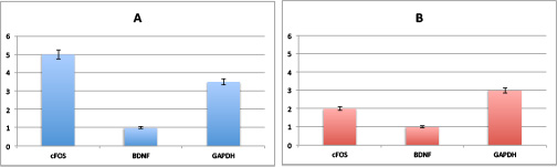
However, can we really say this is true? No! We need error bars!
Both A and B can be thought of as outputs from a random variable.
That is, we can’t make any conclusions from one sample because we
don’t have information on the variance!
Therefore for each transcript we want \(n\) replicates (repeated sampling from the same condition), and would like to calculate the mean and variance.
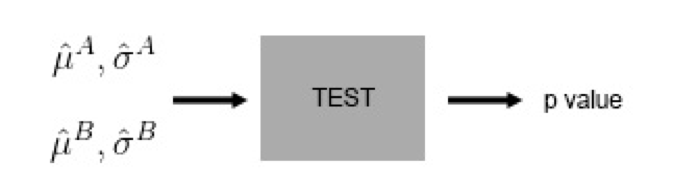
If I have a single transcript x that I am interested in, and I have n replicates in condition A and condition B, then the math looks something like this:
\[\begin{align*} \hat{\mu}^A & = \frac{1}{n}\sum_{i=1}^n X_i^A \\ \hat{\mu}^B & = \frac{1}{n}\sum_{i=1}^n X_i^B. \end{align*}\]We can also estimate sample variances using:
\[\begin{align*} (\hat{\sigma}^A)^2 & = \frac{1}{n-1} \sum_{i=1}^n (X_i^A - \hat{\mu}^A )^2 \\ (\hat{\sigma}^B)^2 & = \frac{1}{n-1} \sum_{i=1}^n (X_i^B - \hat{\mu}^B )^2 \end{align*}\]Statistics side note: the \(\frac{1}{n-1}\) in this formula makes it unbiased!
Now, theoretically more \(n\) is better \(n\), however in real life,
High Throughput Sequencing is expensive and your n costs money!
In the wild, 3 is not an uncommon n, and this creates some problems
because there is an uncertainty in the variance term calculated above as well.
To expand on this – it’s important to note that sigma is an estimate of the true variance, and therefore it too is a random variable! As we know, any random variable has a variance, including the estimated variance – and interestingly, the variance of the estimated variance is significantly bigger than the variance itself (said another way: the variance of the estimated variance is larger than the variance of the mean).
When your \(n = 3\), your variance isn’t accurate! How do we deal with this?
There is a method, which we will discuss in a later lecture.
However – for the sake of continuing, let’s assume we have a reasonable vestimated mu and sigma.
Now we have height and error-bars on our graph, great!
Now all we need is a test to see if transcript 1 is expressed significantly different in the two conditions. The output of this test should give an indication of significant difference, and the magnitude of how significantly different are they?
As it turns out RA Fisher, in 1905 came up with the notion of the p-value, which we’ll be using today.
The p-value is a number between 0-1 and represents the
probability that we reject the null hypothesis, even though it is true.
A p-value is nice in that it requires no modeling of what happens under
the alternate hypothesis. It tests the null hypothesis.
So what is a null hypothesis? To illustrate, we’ll walk through the steps of how to do a T-Test.
How to do a T-Test:
-
Observe data and use it to calculate the T-statistic (more on this coming up)
-
Set the null hypothesis:
a. In our case this is that the distribution of abundances from A and B are the same!
-
Calculate the p-value where \(G(x)\) is the CDF of the distribution of the absolute value of the T-statistic under the null distribution;
the p-value is \(1-G(T)\)a. NB: in some situations the p-value is \(G(T)\) itself depending on what tail of the distribution you’re interested in.
b. What are you computing here? You’re computing the probability that the T statistic exceeds the calculated value
c. Note that when you’re very different – the magnitude of the T value will be large!
Note: Under the null hypothesis, G has a uniform distribution (here’s a cute little proof from a blog if you don’t believe me: p-value proof )
Okay, now how do we calculate our statistic? It’s important to note that there are many statistics other statistics besides the T statistic we will illustrate here, which all make different assumptions and are useful in different situations.
\[T \triangleq \frac{\sqrt{n}(\hat{\mu}^A-\hat{\mu}^A)}{\sqrt{(\hat{\sigma}^A)^2 + (\hat{\sigma}^A)^2}}\]The statistic here is known as the t-statistic and is used for a two-sample t-test. Under the null hypothesis, we assume
\[X_i^A, X_i^B \sim N(\mu, \sigma^2),\]in which case \(p \sim U[0, 1]\), a uniform distribution between 0 and 1.
Fact: \(Y\) with cdf \(F(y) \triangleq \text{Pr}(Y \leq y)\), then \(F(Y) = Z U[0, 1]\).
We can use such a test to determine if the mean value of a transcript is the same between conditions A and B based on the p-value obtained. While we only described one statistic here, there are several types of statistics one could use depending on the assumptions one would like to make on the null hypothesis (e.g. non-equal variance).
If we have a small p-value, then we are more interested in the transcript we’ve made a discovery! It is unlikely that we saw this difference and the distributions are actually the same (\(i.e.\) they belong to the null).
Multiple testing
What is the threshold at which we think we’ve made a discovery?
According to RA Fisher, 0.05 is a good threshold.
This means that there’s only a 5% chance that the T statistic
we observed was actually from the null distribution. However,
when RA Fisher invented this test he was testing only one hypothesis,
not ~30k hypotheses like we are with RNAseq!
When we have 30k hypotheses, false positives become an issue!
That is to day, by random chance, you will see some transcripts
that look positive just due to random fluctuations. By definition,
the p-value of 0.05 represents the chance that we will reject the null
hypothesis when it is actually true. If we do this 30k times, this means
we will have ~1.5k false positives! Therefore you can’t use 0.05 on
each test independently!
This then brings us to the last portion of differential analysis.
You’re not just testing one hypothesis; you’re testing many in parallel.
You’re also not testing the hypotheses against teach other, just doing many
tests!
Framing this in terms of discoveries – we then have 2 types of possible discoveries under this type of analysis:
-
True discoveries (TDs)
-
False discoveries (FDs)
We need a procedure to keep our False Discoveries low so we don’t have any Fake News!

Let’s say \(V\) is our number of FDs. If we do m tests, and make \(R\) discoveries, some of those discoveries will be FDs
One way of controlling \(V\), is to make sure that the probability
of having \(1\) or more FD is very small.
So instead of the threshold \(0.05\)
for each individual test, let’s require a
p-value of less than \(0.05\), such that \(V\) is controlled in regards to the
\(m\) tests we’re about to do. This is called controlling
the family-wise error rate (FWER):
How do I change the threshold to satisfy this final goal?
The answer is that we need to bound this probability – and we can calculate a direct bound w/o assuming independence of the individual tests.
For each test, what is the probability that we make a FD? Let’s call this FD1, FD2, FD3, etc. Then, by union bound, the probability that we make at least one FD is bounded by the sum of the FD probabilities of each test: FD1, FD2, FD3, etc.
We make a discovery when our p-value is less than theta, which is our more stringent criteria than 0.05.
We then ask, with what theta is the probability I reject the null less than \(0.05\), and we can make our lives easier by noting that since p is uniformly distributed, theta is the probability of making a FD.
Therefore, the upper bound is the union of all events
\[\begin{align*} \text{Pr}[V \geq 1] & \leq m \theta \leq 0.05 \\ \implies \theta & = \frac{0.05}{m} \\ & = 5 * 10^{-6} \end{align*}\]So if m is \(10,000\) our adjusted theta p-value becomes \(5x10⁻⁶\)!
This is called a Bonferroni Correction, and \(P(V >0)\) is called the
family wise error rate (FWER).
We then set the threshold for discovery to be \(5x10⁻⁶\) and we’re in business!
However this is a very conservative threshold -> it’s very hard to write up a
paper with this number, we’re unlikely to get such a small p-value.
This then leaves us with a problem: This condition is too stringent…
Let’s re-visit our prerequisites then. Is it really so bad to make a False Discovery? According to a well cited Benjamini-Hochberg paper in 1995, we can relax our expectation that we never make a false discovery, as long as proportional to all our real discoveries, the false discoveries are small.
As above, let R be the total number of discoveries.
We then define a False Discovery Proportion (FDP) such that
where \(V\) is still our number of FDs.
It’s okay for \(V > 1\) as long as it is smaller than \(R\) – that is to say as long as we keep our FDR < 5% we still find a good number of targets to chase and don’t waste NIH money too much.
However you should be aware that this is just \(V/R\) is still a
random variable – and the data generated from a random process is also random.
We can’t guarantee the random variable is less than a threshold for sure.
So the FDR is actually defined to be the expectation of this random variable:
\[\text{FDR} \triangleq E \left[ \frac{V}{\max(1,R)} \right].\]Note: we assume \(R\) is nonzero. Thus replace \(R\) by \(\max(R,1)\).
This is less conservative, and will actually get us some reasonable data to work with, yay!
So how do you control FDR to be less than \(5\%\)? You define a new metric and procedure to guarantee that the FDR is less than \(5 \%\), which we will explore next lecture!
This and the next few lectures on differential expression analysis borrow a lot of material from a lecture in the Computational Genomics Summer School at UCLA in 2017 by Prof. Lior Pachter of CalTech (and one could say were inspired by it).