Lecture 9: Alignment - Dynamic Programming and Indexing
Lecture 9: Alignment - Dynamic Programming and Indexing
Tuesday 6 February 2018
Topics
In the last lecture, we introduced the alignment problem where we want to compute the overlap between two strings. Today we will talk about a dynamic programming approach to computing the overlap between two strings and various methods of indexing a long genome to speed up this computation.
Review of alignment
When working with reads, we are generally interested in two types of alignment problems.
- Reference-based SNP/variant calling, where reads are aligned to a reference. We are often interested in computing the alignment for a billion reads to a long reference genome.
- De novo assembly, where reads are aligned to each other
To compute the optimal alignment between to genomic sequences (or more generally strings), we can find the minimal edit distance between the two sequences. We note that for both of the above problems, a lot of computation is repeated using the same data. As a recap, the figure below finds the minimal edit distance alignment between two strings X = ‘GCGTATGTG’ and Y = ‘GCTATGCG’. Recall that for the standard edit distance problem, we assign a substitution, deletion, or insertion equal penalties.
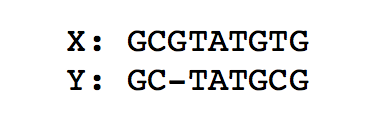
To go from X to Y, we need at least one deletion and one substitution. Therefore the edit distance is 2.
Dynamic programming
Dynamic programming is the strategy of reducing a bigger problem into multiple smaller problem such that solving the smaller problems will result in solving the bigger problem. First, we need to define the “size” of a problem. For edit distance, we let \((i,j)\) represent the problem of computing the edit distance between \(X^i\) and \(Y^j\). \(X^i\) is the length-\(i\) prefix of the string \(X\), and \(Y^j\) is the length \(j\) prefix of string \(Y\). If we let \(m\) represent the length of \(X\) and \(n\) represent the length of \(Y\), then the edit distance between \(X\) and \(Y\) is the solution to problem \((m,n)\). The claim is: if we can solve all the \((i,j)\) problems for \(0 \leq i \leq m\) and \(0 \leq j \leq n\) except \(i=m\) and \(j=n\), then we will efficiently obtain a solution for problem \((m,n)\).
Let \(D(i,j)\) equal the edit distance between \(X^i\) and \(Y^j\). Suppose we are looking at \(X^3\) = ‘GCG’ and \(Y^2\) = ‘GC’. The edit distance between these two is 1. To express this as even smaller problems, we need a key insight: problem \((i,j)\) can be solved directly using the solutions from 3 subproblems:
- \((i-1,j)\), where we advance \(X\) by one character and put an empty symbol in \(Y\).
- \((i,j-1)\), where we advance \(Y\) by one character and put an empty symbol in \(X\)
- \((i-1,j-1)\), where we advance both \(X\) and \(Y\) by 1 character.
Since we are interested in the minimal edit distance,
\[D(i,j) = \min\{D(i-1,j)+1, D(i-1,j-1) + 1, D(i-1,j-1)+ \delta(X[i],Y[j])\}\]where \(\delta\) represents an indicator function
\[\delta(a,b) = \begin{cases}1 & \text{if } a\neq b,\\ 0 & \text{otherwise.}\end{cases}\]Thus \(\delta(X[i],Y[j])\) is 1 \(i\)th character of \(X\) is is the same as the \(j\)th character of \(Y\), and 0 otherwise.
We can think of solving this problem as filling in the entries of a table where the columns correspond to the empty string \(\emptyset\) plus the characters in \(X\), and the rows corerspond to the empty string plus the characters in \(Y\). Please see the figure below for the filled out table corresponding to the first example in this lecture.
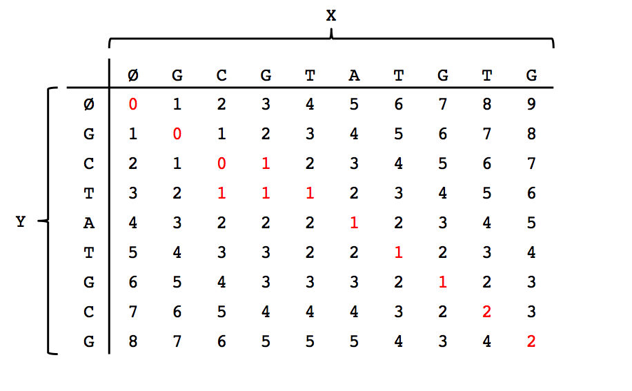
Note that the \((m,n)\)th entry (bottom-right corner) indeed has the minimal edit distance between the two strings. After filling out the dynamic programming table, we can trace a path back from the bottom-right entry to the top-left entry along the smallest values to obtain our alignment shown in the first figure in this lecture.
Each computation requires looking up at most 3 entries of the table. Therefore the complexity of this algorithm is \(O(mn)\). For read-overlap graph assembly, we have \(N\) reads each of length \(L\). Using this edit distance approach, we will need \(O(N^2L^2)\) operations to perform assembly. With \(N\) possibly the order of \(10^8\) or \(10^9\) for a sequencing experiment, this operation is quite expensive.
For variant calling, we want to align \(N\) reads to a reference genome of length \(G\). Computing the edit distance between a read and the genome is \(O(LG)\). The runtime is \(O(NLG) = O(cG^2)\) where \(c\) is the coverage depth. \(G\) can be large (\(3\times 10^9\) for the human genome) and therefore this operation is also quite expensive.
Genome indexing
The genome is very long, so alignment algorithms that require a search along the entire genome (for every read) seem suboptimal. We can use an index to store the context of the genome to make the search more efficient, reducing the amortized cost.
Error free case
We first consider the idealistic case. Suppose each read is error-free; the reads come directly from the genome. Every read has a location in this genome, and we want to find this location fast. We can build a sorted list of \(L\)-mers (each read is length \(L\)) such that we can easily look up the genome indices of specific \(L\)-mers. We build the list by extracting all length \(L\) sequences from the genome and ordering the sequences in lexicographical order. For each new read coming in, we can quickly search for the corresponding \(L\)-mer key in the list, obtaining its location in the genome.
Since the list is at most length \(G\), doing a binary search on the list is \(O(\log G)\). Note that the complexity of building the index is \(O(G)\), but we only have to build this index once. Looking up \(N\) reads is \(O(N \log G)\). Overall, the total cost is \(O(G + N \log G)\), much better than \(O(G^2)\).
Rather than using a sorted list, we could also use a hash table. This results in \(O(1)\) lookup for new reads, but keeping the entire hash table in memory is more expensive.
Low error case
We now look at the regime where the reads often differ slightly from the reference, either due to low-frequency errors (e.g. less than 1%, in the case of Illumina reads) or SNPs. Recall from last lecture that when the error is low, we typically get 0-2 errors per length-100 read. We will see many length-20 subsequences which are error free. So instead of making a sorted list with \(L\)-mers, we can create a sorted list of \(20\)-mers. With this strategy, \(20\)-mers with errors will map to a random location or no location at all. This is not an issue, however, because if 20 is a reasonably large number, then most random reads will map to no location in the genome.
Indexing in practice
The seed-and-extend concept is based on this fingerprinting approach. We starting by finding seed locations using k-mers, and use these to identify potential matching regions in the genome. Then one aligns using the dynamic program in these regions. Almost all practical tools use this approach.
In the low-error case, tools used in practice use short subsequences (of length 20-30) as potentially error-free fingerprints for looking down potential alignment locations. Given a read they find hash matches for each 20-mer in the read, tools like Bowtie compute a set of potential locations a read could match. They then compute alignments by dynamic programming in those locations. Some tools like Kallisto take an intersection of the set of potential matches returned by the k-mers in a read (shifted appropriately) to obtain locations in the reference the reads could have come from. (The actual algorithm is a little more subtle where the intersection is taken only between k-mers that have an entry in the hash table. The underlying assumption is that k-mers with 1-2 errors will not appear anywhere else in the reference.)
Read overlap graph approaches typically require \(O(N^2)\) operations where \(N = 10^8\) or \(10^9\). We can use the fingerprinting idea to alleviate some of the cost. We can build a table where the keys are \(k\)-mers and values are the reads containing a particular \(k\)-mer. We build this table by scanning through all the reads and applying a hash function. Now, for each read, we want to find a bunch of other reads that may align to the query read. Using this hash strategy gives us far less “candidate” reads per read, saving significant computation. The actual savings will depend on the number of repeats, but the cost reduces from \(O(N^2)\) to \(O(aN)\) for some constant \(a \ll N\). This is done in practice by assemblers like DAligner, Minimap and MHAP.
High error case and the MinHash
If the error rate is high, we can use the same approach as the low-error case by reducing the size of the \(k\) corresponding to the \(k\)-mer used for indexing. If the error is high enough (15% in the case of PacBio reads), \(k\) will need to be small to ensure a high probability of errors mapping to no location on the genome. With a smaller \(k\), we also expect more collisions in our table, since the set of unique \(k\)-mers is smaller. More collisions results in a more expensive alignment procedure.
When building the read overlap graph in the regime of high read errors, we can leverage minhashing to efficiently filter read pairs that need to be aligned. This is the approach used by MHAP. We first consider two sets \(A, B\). We define the Jaccard similarity between the two sets as
\[J(A, B) = \frac{| A \cap B |}{|A \cup B |}\]or the size of the intersection of the two sets divided by size of the the union of the two sets. When comparing two genomic reads, we can cut the two sequences up into overlapping k-mers, just like before. Each genomic read can be represented by a set of k-mers. If two reads are similar, then the Jaccard similarity of their k-mer set representations should be relatively close to 1. To compute the Jaccard similarity exactly, this boils back down to the alignment issue. Minhash allows us to approximate the Jaccard similarity with small computation. We define a hash function \(h\) that maps each element in \(A \cup B\) to some integer. This hash function also has some pseudo-random property, meaning that it assigns random values to different inputs (but assigns the same value for the same input). We can apply the hash function to all the objects in \(A\) (corresponding to our first read) and \(B\), resulting in
\[h_\text{min} (A) = \min_{x \in A} h(x).\]Note that
\[Pr[h_\text{min}(A) = h_\text{min}(B)] = \frac{|A \cap B|}{|A \cup B|}.\]To see this, note that \(h_\text{min}(A) = h_\text{min}(B)\) occurs if and only if the \(x\) that achieves the minimum hash value is in \(A \cap B\). The probability that this occurs is exactly the Jaccard similarity between \(A\) and \(B\). We apply a small set of different hash functions \(h_1, \dots, h_K\) and observe the frequency with which \(h_\text{min}(A) = h_\text{min}(B)\). This gives us an unbiased estimate of the Jaccard similarity. The larger the value of \(K\), the more accurate the estimate is, but the more expensive the computation.
Minhashing is a more general technique that can be applied whenever finding the distance between two sets is relevant (e.g. mining datasets). Some applications are listed here.