Lecture 7: Assembly - De Bruijn Graph
Lecture 7: Assembly - De Bruijn Graph
Tuesday 30 January 2018
Topics
- Interleaved Repeats
- de Bruijn Graphs
- Dense Read Model and the L-spectrum
- de Bruijn algorithm
- Examples - A practical algorithm based on the de Bruijn graph algorithm
- Simple Bridging
Interleaved Repeats
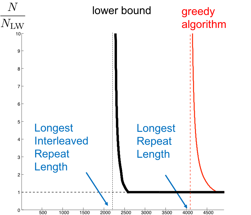
We ended the last lecture with a discussion on the following plot:
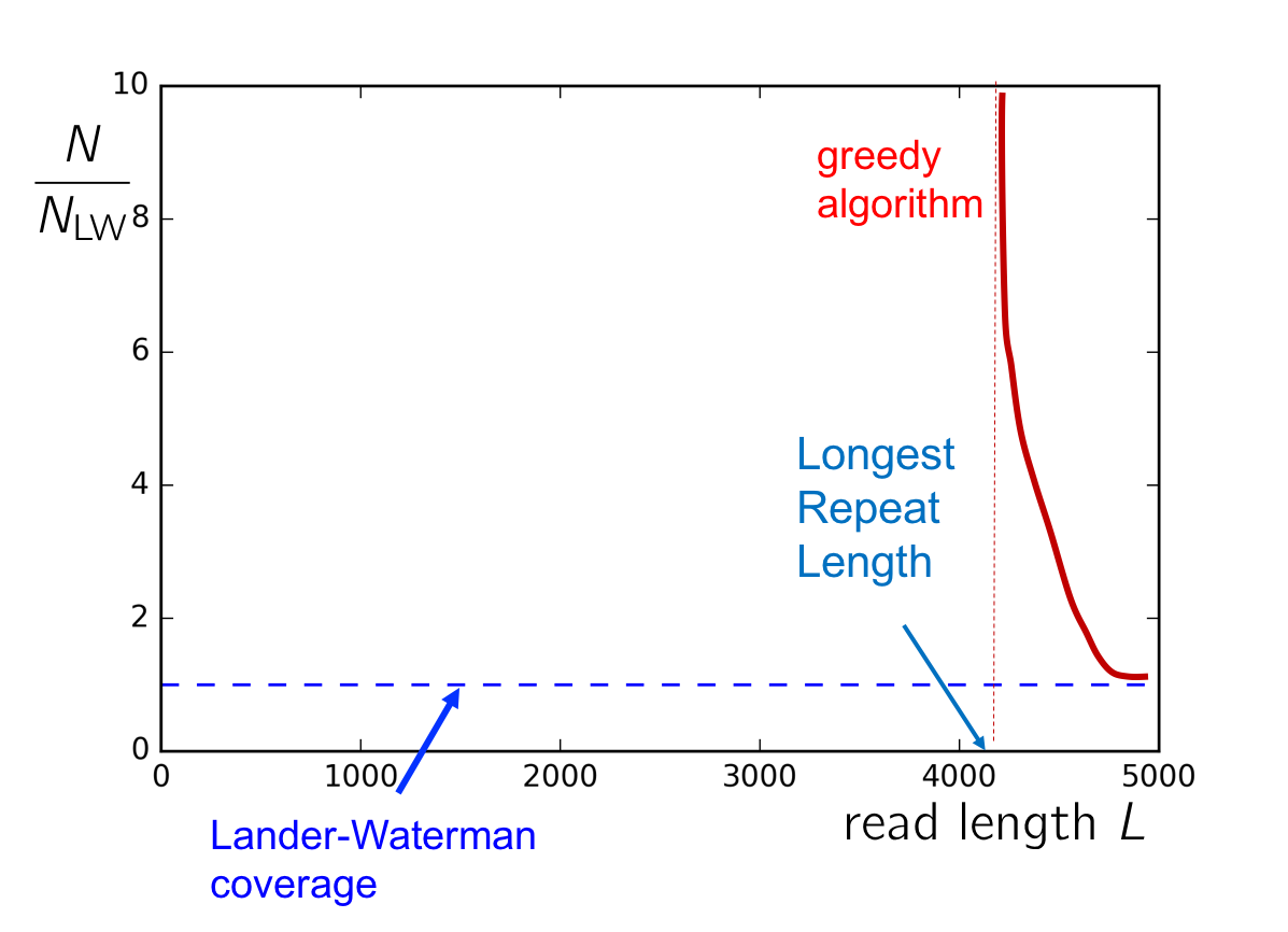
If the coverage \(c\) and the length of the longest repeat \(\ell_\text{repeat}\) lies in the top right quadrant, then the Greedy Algorithm will succeed with high probability. In particular, we note the greedy algorithm fails if the read length is smaller than the length of the longest repeat in the genome. In this section, we derive a genome-dependent lower-bound on both the read length and number of reads required for successful assembly.
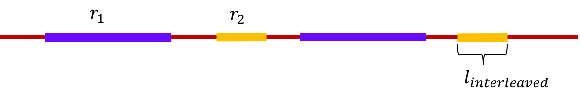
A pair of repeats are said to be interleaved if they appear alternately in the genome. The length of the shorter of two interleaved repeats is called the length of the interleaved repeat. For example, in the figure below, \(r_1\) and \(r_2\) are interleaved repeats, and the length of the interleaved repeat is the length of \(r_2\). Note that if the reads are shorter than the length of the shorter repeat, then we cannot determine the order of the two regions between the two repeats.
An interleaved repeat is said to be bridged if at least one copy of one of the repeats is bridged.
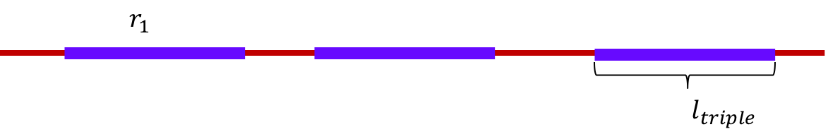
A triple repeat is a repeat that appears thrice in the genome. This is a special case of an interleaved repeat. This is illustrated below.
Theorem [Ukkonen 1992; Bresler, Bresler, and Tse 2013]: Assembly of a genome is impossible if any interleaved repeat is not bridged.
As a corollary, we note that this theorem means that at least one copy of a triple repeat needs to be bridged for assembly of a genome to be feasible.
Proof by picture
Using calculations almost identical to those used in quantifying the performance of the greedy algorithm, we can derive a curve showing the number of reads necessary for successful assembly in a given genome. This is shown for an example genome below
de Bruijn graphs
Dense Read Model and the L-spectrum
To come up with an algorithm that performs better than the greedy algorithm, we first take a detour. We consider an idealized setting called the dense read model. Trying to solve the assembly problem in this setting gives us an algorithm which we can then modify for the shotgun sequencing case.
A dense read model assumes that we have a read starting at every position in the genome. The multi-set of reads thus obtained is called the L-spectrum.
This is illustrated below.
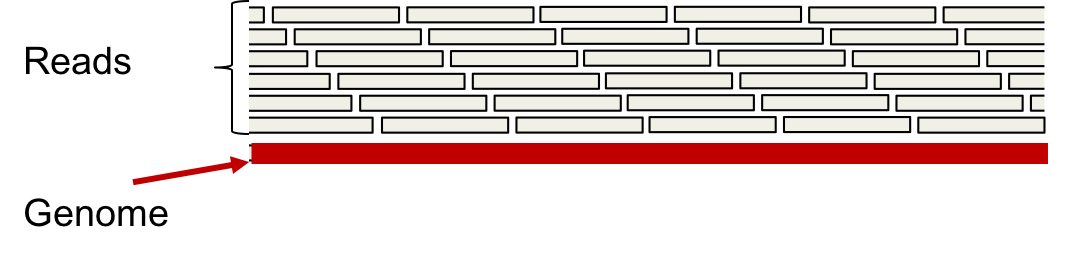
The L-spectrum can be thought of as the set of all unique length-L reads we obtain when we have infinitely many reads from the genome \(\mathcal{G}\) (unique in terms of position).
de Bruijn algorithm
In graph theory, the standard de Bruijn graph is the graph obtained by taking all strings over any finite alphabet of length \(\ell\) as vertices, and adding edges between vertices that have an overlap of \(\ell-1\). In the following, we consider assembly using a slightly modified version of the standard de Bruijn graph from the L-spectrum of a genome.
Given the L-spectrum of a genome, we construct a de Bruijn graph as follows:
-
Add a vertex for each (L-1)-mer in the L-spectrum.
-
Add \(k\) edges between two (L-1)-mers if their overlap has length L-2 and the corresponding L-mer appears k times in the L-spectrum.
An example de Bruijn graph construction is shown below.
We note that an Eulerian path in the de Bruijn graph corresponds to a sequence consistent with an L-spectrum. Thus if a de Bruijn graph corresponding to the L-spectrum of a genome has a unique Eulerian path, then a genome can be assembled from its L-spectrum. Finding the Eulerian path is an easy problem, and there exists a linear-time algorithm for finding it. This assembly approach via building the de Bruijn graph and finding an Eulerian path is the de Bruijn algorithm.
Theorem [Pevzner 1995]: If L, the read length, is strictly greater than \(\max(\ell_\text{interleaved}, \ell_\text{triple})\), then the de Bruijn graph has a unique Eulerian path corresponding to the original genome.
This gives us Ukkonen’s lower bound, and successful assembly can be achieved as the number of reads become arbitrarily large.
Examples
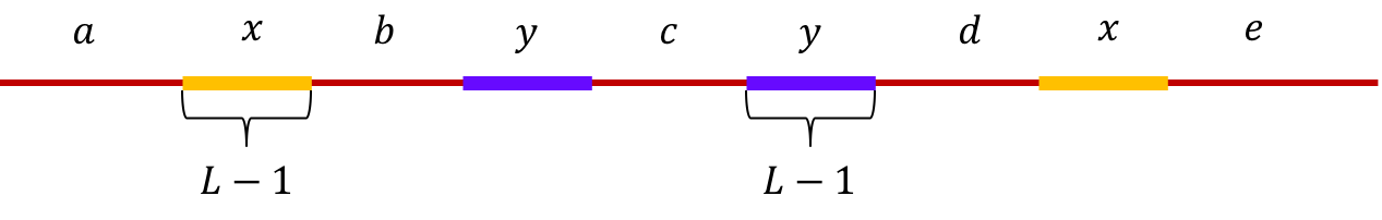
Example 1 (Interleaved repeats of length L-1): Let \(x\) and \(y\) be two interleaved repeats of length L-1 on the genome. Let us assume that the genome has no other repeat of length L-2 or more. We show the genome using the shorthand: \(\mathtt{a-x-b-y-c-x-d-y-e}\). This is illustrated below.
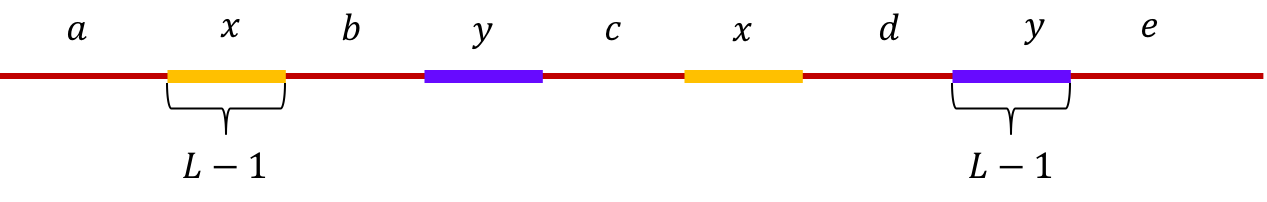
The de Bruijn graph from the L-spectrum of this genome is given by
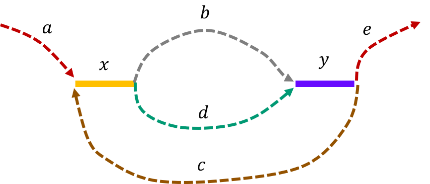
We note that an Eulerian path on the graph would start from \(\mathtt{a - x}\). Then one can either leave \(\mathtt{x}\) through \(\mathtt{b}\) or \(\mathtt{d}\) to get to \(\mathtt{y}\). Any Eulerian path then has to take the path \(\mathtt{c}\) to \(\mathtt{x}\). Then we can take the path not taken from \(\mathtt{x}\) last time to get to \(\mathtt{y}\). This gives us two genomes consistent with the de Bruijn graph : \(\mathtt{a-x-b-y-c-x-d-y-e} \text{ and } \mathtt{a-x-d-y-c-x-b-y-e}\text{.}\)
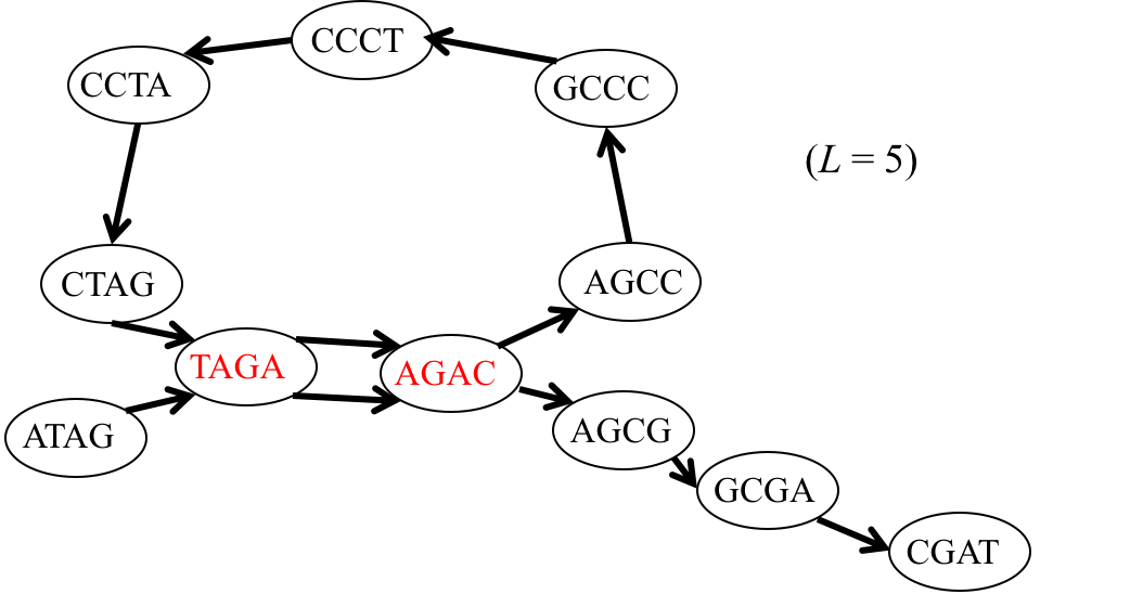
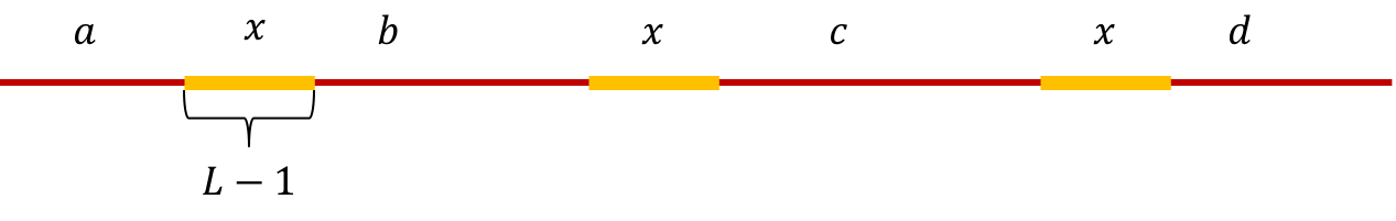
Example 2 (Triple repeats of length L-1): Let \(x\) be triple repeats of length L-1 on the genome. Let us assume that the genome has no other repeat of length L-2 or more. The genome will be represented using the shorthand: \(\mathtt{a-x-b-x-c-x-d}\). This is illustrated below.
The de Bruijn graph from L-spectrum of this genome is given by
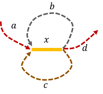
We note that that an Eulerian path on the graph would start from \(\mathtt{a - x}\). Then one can either leave \(\mathtt{x}\) through \(\mathtt{b}\) or \(\mathtt{c}\) to get back to \(\mathtt{x}\). The path then leaves \(\mathtt{x}\) using the other path out to return a third time to \(\mathtt{x}\). Finally, the path leaves \(\mathtt{x}\) through \(\mathtt{d}\). This gives us two genomes consistent with the de Bruijn graph: \(\mathtt{a-x-b-x-c-x-d} \text{ and } \mathtt{a-x-c-x-b-x-d.}\)
In both these examples we have that \(L-1= \ell_{\text{interleaved}}\) , and thus genome can not be assembled from the L-spectrum as stated in the necessary condition of the theorem. Next let us look at examples where the L-spectrum can be used to assemble the genome by the de Bruijn graph algorithm, giving some intuition why the condition is also sufficient.
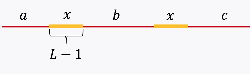
Example 3 (Simple repeat of length L-1): Let \(x\) be simple repeats of length L-1 on the genome. Let us assume that the genome has no other repeat of length L-2 or more. The genome will be represented using the shorthand: \(\mathtt{a-x-b-x-c}.\)
The de Bruijn graph from L-spectrum of this genome is given by
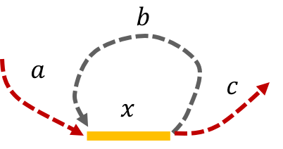
It is easy to see that the only Eulerian path on this de Bruijn graph is the one corresponding to \(\mathtt{a-x-b-x-c}.\) Note that the greedy algorithm may have chosen the path \(\mathtt{a-x--c}.\)
Example 4 (Non-interleaved pair of repeats of length L-1): Let \(x\) and \(y\) be two non-interleaved repeats of length L-1 on the genome. Let us assume that the genome has no other repeat of length L-2 or more. We show the genome using the shorthand: \(\mathtt{a-x-b-y-c-y-d-x-e}\).
The de Bruijn graph from L-spectrum of this genome is given by
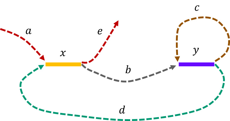
It is fairly easy to show that \(\mathtt{a-x-b-y-c-y-d-x-e \ \ }\) is the only Eulerian path in the de Bruijn graph.
A practical algorithm based on the de Bruijn graph algorithm
We note that the de Bruijn graph algorithm would work if we had the L-spectrum of a genome and \(L-1 > \ell_{\text{interleaved}}\). However the number of reads of length \(L\) necessary to get the L-spectrum would be astronomical even for modest genome sizes and large read lengths. Therefore coverage alone is not enough.
To get a more practical version of the de Bruijn graph algorithm, we introduce the concept of k-coverage where each substring of length k is contained in at least 1 read. We basically try to get the k-spectrum of a genome from reads of length L where L > k. Each read of length L gives us L-k+1 strings of length k (called k-mers). To quantify the number of reads necessary for this to work, given a success probability \((1-\epsilon)\), we must characterize the number of L length reads necessary to get the k-spectrum.
Note that to get k-coverage, for every read there exists a second read with its starting position within L-k+1 positions after the starting position of the first genome. Note that a set of reads k-covering a genome implies that one can recover the k-spectrum of the genome from the reads (Can you see why?).
Consider the following practical algorithm to assemble:
Sample reads enough to get k-coverage.
Run the de Bruijn graph algorithm with the k-spectrum thus obtained.
Here we note that k is a tradeoff parameter. For the algorithm to succeed we need that k - 1 > \(\ell_{interleaved}\), the length of the longest interleaved repeat. Thus a larger k makes assembling more genomes possible; however, larger values of k lead to smaller values of L-k+1. k coverage tells us that we need to get a read starting in every L-k+1 window of the genome, so one would need to sample more reads.
Using similar calculations to those used in the last lecture, we get the following graph describing the number of reads necessary for an algorithm to succeed.
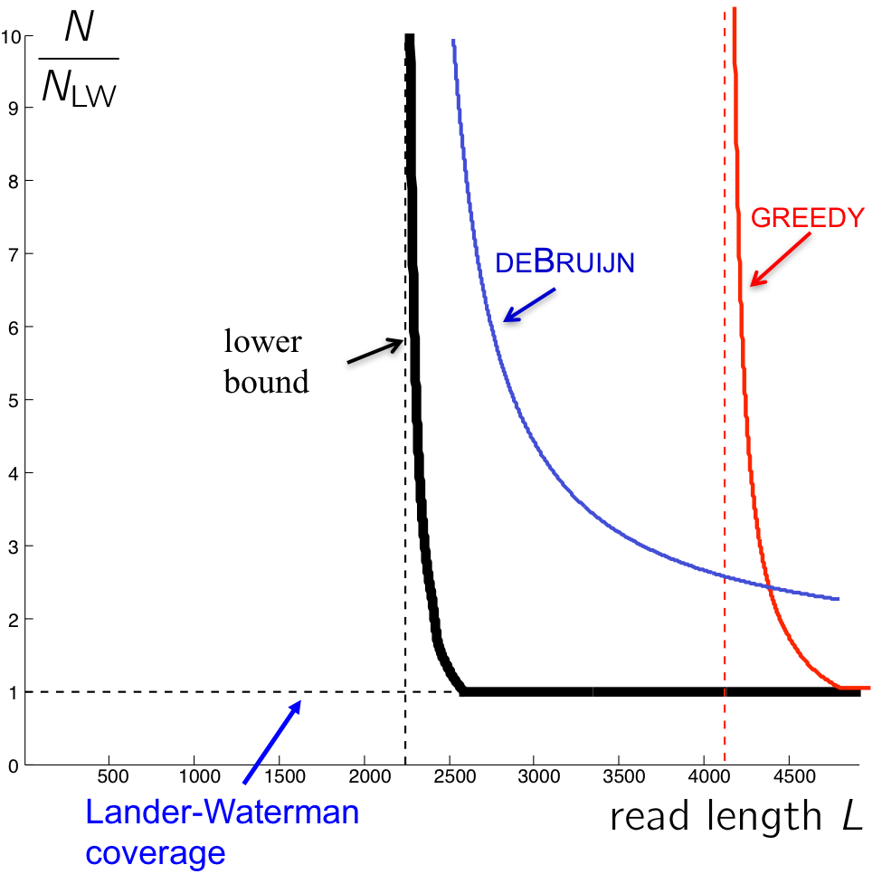
The curve for the de Bruijn algorithm is computed by setting \(k = \ell_{interleaved} + 1\), thus it is the most optimistic performance achievable, since in reality the algorithm does not know \(\ell_{interleaved}\) and has to be more conservative. We note that though the de Bruijn graph algorithm achieves the vertical asymptote, it does need a fairly large number of reads to do so. Although greedy has a worse vertical asymptote, it is better for larger values of L since it requires less reads.
We note that there still exists a gap between the de Bruijn curve and the lower bound. This is because the algorithm requires every \(\ell_{\text{interleaved}}\)-mer on the genome to be bridged (Note that k-coverage means every k-2 mer in the genome must be bridged. Why?) rather than just having the interleaved repeat bridged.
Simple Bridging
By taking advantage of the fact that we do not need to bridge all interleaved repeats with k-mers, we can come up with modified versions of the de Bruijin algorithm. We set k \(<< \ \ell_{\text{interleaved}}\), and we do something special for the long interleaved repeats, which are few in numbers.
The problem we had when k \(\leq \ell_{\text{interleaved}}\)+ 1 was that we have confusion when finding the Eulerian path when traversing through all the edges, as covered in the previous lecture (Refer to examples of de Bruijin graphs in Lecture 8). When multiple Eulerian paths exist, we cannot guarantee a correct reconstruction.
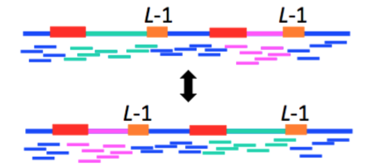
We can circumvent this problem by using the reads (L-mers) themselves to resolve the conflicts. In the figure below, with k < \(\ell_{\text{interleaved}}\), there were two potential Eulerian paths: one traverses the green segment first and the other traverses the pink segment first.
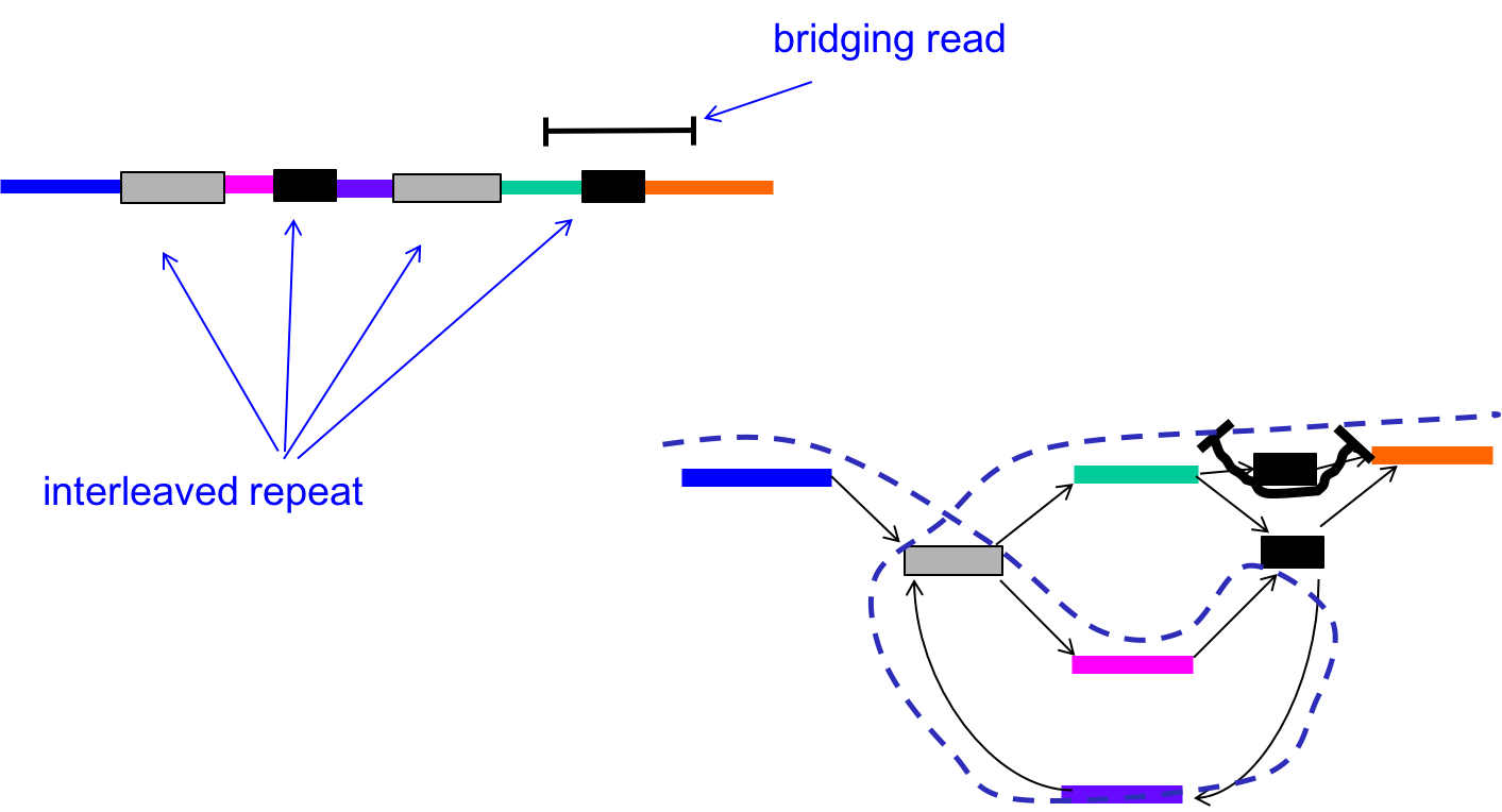
By incorporating the information in the bridging read, however, we can reduce the number of Eulerian paths to one. In other words, we can resolve the ambiguity in the graph as follows:
- Find the bridging read on the graph, in this case on the top right.
- Since we know that the orange segment must follow the green segment, replicate the black node and create a separate green - black - orange path.
Information from bridging reads simplify the graph.
At this point, our conditions for a successful assembly is as follows:
- All interleaved repeats (except triple repeats) are singly bridged.
- k-1 > \(\ell_{\text{triple}}\) (length of the longest triple repeat).
The performance of this algorithm is shown in the figure below. We also include the performance of the multibridging algorithm, an extension of simple bridging algorithm.
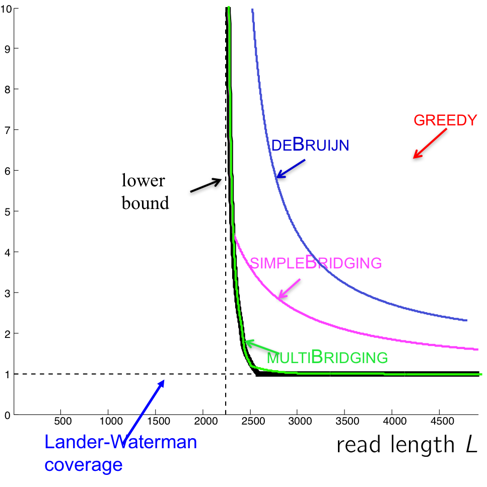
There still exists a small gap between the multibridging algorithm and the lower bound. The process of closing this gap is closely tied with showing that P = NP, a famous (perhaps the most famous) unsolved problem in theoretical computer science. We will take a closer look next lecture.