Lecture 6: Assembly - Greedy Algorithm
Lecture 6: Assembly - Greedy Algorithm
Thursday 25 January 2018
Topics
Coverage analysis
Recall that we are interested in assembling a genome from individual reads. Last time, we showed that the number of reads covering a particular location \(i\) is roughly Poisson with parameter \(c\), the coverage depth. We have
\[\begin{align*} G &= \text{Length of the genome},\\ L &= \text{Read length},\\ N &= \text{Number of reads}, \\ c &= NL/G = \text{Coverage depth}. \end{align*}\]Let \(Y_i \in \{0, 1\}\) represent the event that the \(i\)th base is covered. While \(\text{Bin}(N, L/G)\) is a natural distribution for \(Y_i\), we note that in practice \(L/G\) is very small, and therefore we can approximate this binomial distribution with \(\text{Poiss}(c)\):
\[\begin{align*} Pr(Y_i = 0) = \left(1-\frac{L}{G}\right)^N \approx \left( e^{-L/G}\right)^N = e^{-c}. \end{align*}\]What is the probability that at we do not achieve coverage? In other words, what is the probability that at least one base is not covered? We can let \(X\) represent the number of bases not covered. Then
\[\begin{align*} E[X] = G. \end{align*}\]The event of coverage for each base is not independent, but the expectation can be computed due to the linearity property of expectation.
\[\begin{align*} Pr(\text{lack of coverage}) &= Pr(X \geq 1) \\ &\leq E[X] \text{ (by the Markov inequality)} \\ &= Ge^{-c} \end{align*}\]If we let \(\epsilon = Ge^{-c}\), our desired maximum probability of lack of coverage, then
\[c = \ln \frac{G}{\epsilon}.\]This value of \(c\) is known as the Lander-Waterman coverage. We note that for successful assembly, we need to constrain \(L\) somehow. The number \(\ln\frac{G}{\epsilon}\) does not depend on the genome (only its length), but \(L\) intuitively should depend on the actual sequence of the genome. One can imagine that for more complex genomes, we need a larger \(L\) for successful assembly. Additionally, assembly should generally be impossible for \(L=1\). But how do we measure the complexity of the genome?
Greedy algorithm
Assume that the reads are perfectly clean (no errors in the characters of the read). We begin by discussing a natural algorithm for assembling the genome de novo from reads: repeatedly find a pair of sequences that have a large amount of overlap and merging the two sequences into one longer sequence. The sequences are initialized to be the observed reads.
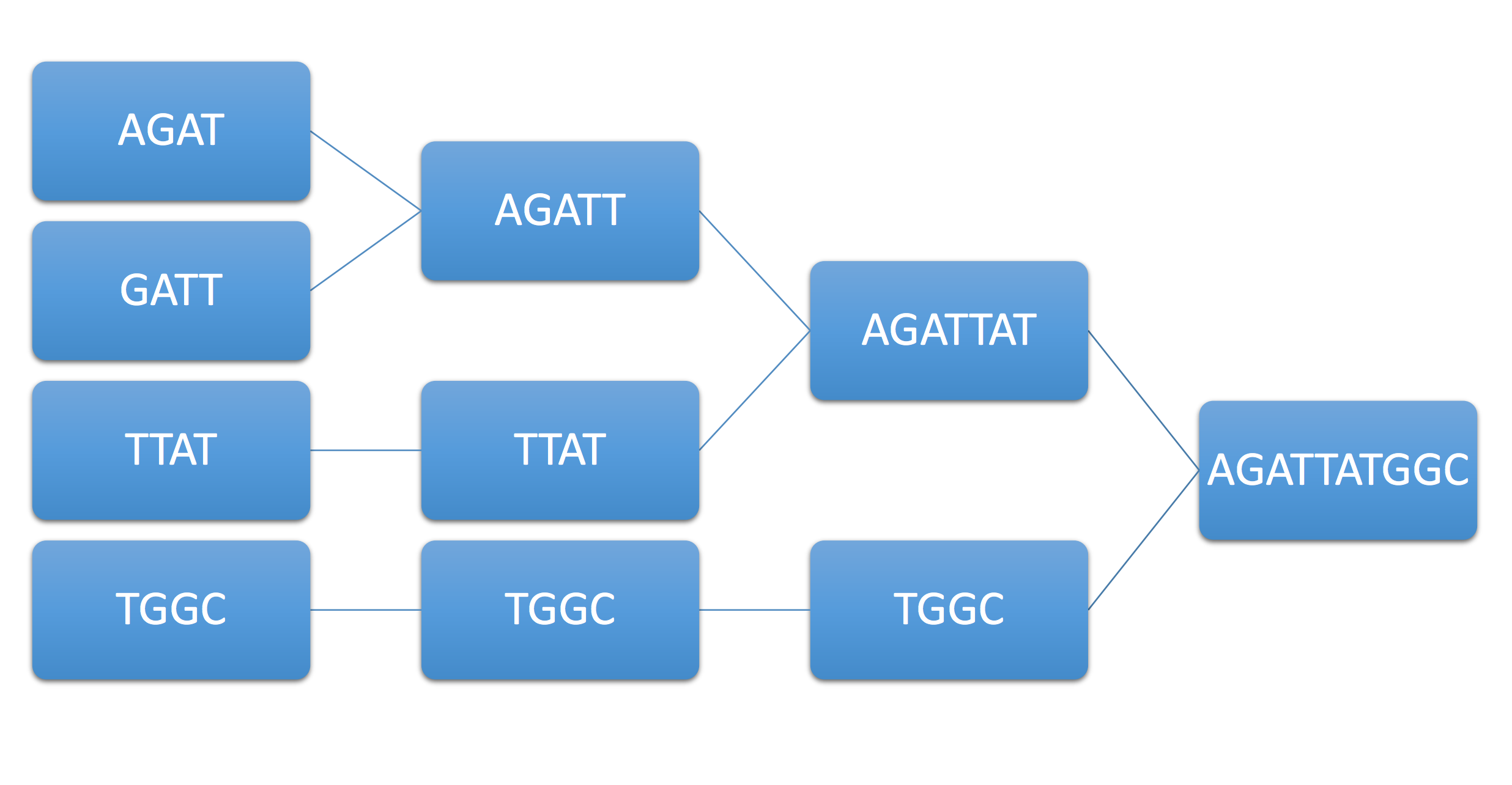
Example 1. Consider the example genome AGATTATGGC and its associated reads AGAT, GATT, TTAT, TGGC. The following figure summarizes this procedure, known as the greedy algorithm.
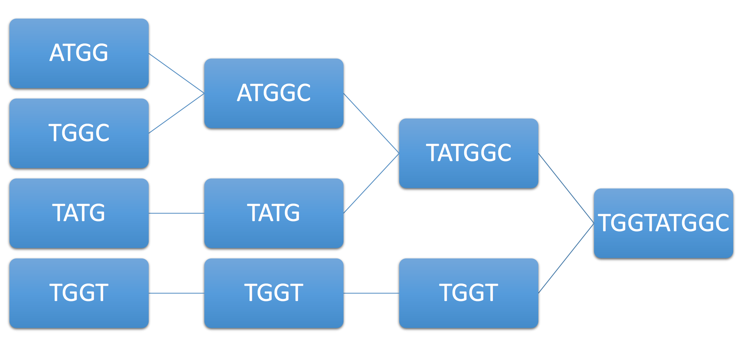
Example 2. As another example, consider the example genome ATGGTATGGC and its associated reads ATGG, TGGT, TATG, TGGC. Immediately, we see that ATGG can be merged with either TGGT or TGGC (ambiguity). Let’s say the algorithm chooses TGGC, resulting in the following final sequence:
Note that although we have achieved coverage and each base is covered by at least one read, the greedy approach can still fail. Can we guarantee under some condition on the genome that the greedy algorithm succeeds? We assume that the read length is fixed based on the technology used.
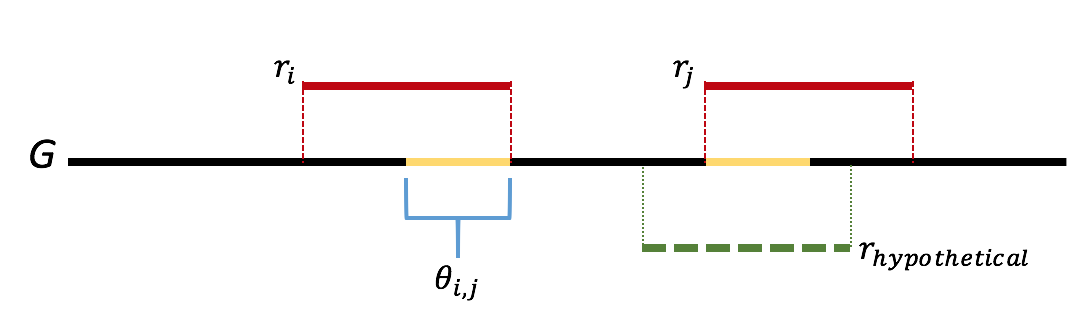
We will attempt to form an argument by contradiction. One can think of the greedy algorithm as behaving in the following way: we start by looking for length-\(\ell\) overlaps. If we do not find anything, then we look for length \(\ell-1\) overlaps. Let \(\ell\) be the first step where we we incorrectly merge two reads. Let \(r_i\) and \(r_j\) be the two reads incorrectly merged. Let \(\theta_{i,j}\) be the overlap between reads \(r_i\) and \(r_j\). We further note that the greedy nature of the algorithm means that all overlaps of length greater than that of \(\theta_{i,j}\) are already merged. We note that this means that the sequence \(\theta_{i,j}\) appears twice in the genome. Further we note that if either copy of \(\theta_{i,j}\) was bridged, meaning that there exists a read that completely overlaps the copy by at least one base on each side, then one of \(r_i\) or \(r_j\) would have had a overlap longer than the length of \(\theta_{i,j}\), which we would have merged first. This gives us that \(\theta_{i,j}\) is not bridged, which is contradiction. Therefore there is never an incorrect merge in the algorithm. This argument is illustrated in the figure below.
A sufficient condition for reconstruction is: all repeats are bridged. In example 2, we see that the length-4 repeat ATGG cannot possibly be bridged by length-4 reads.
We have proved the following theorem:
Theorem. Let a set of reads from a genome fully cover the genome. Moreover, let each repeat in the genome be bridged by at least one read, that is there exists a read that starts at least one base before every repeat, and ends at least one base after. Then the greedy algorithm is guaranteed to reconstruct the original DNA in the absence of noise.
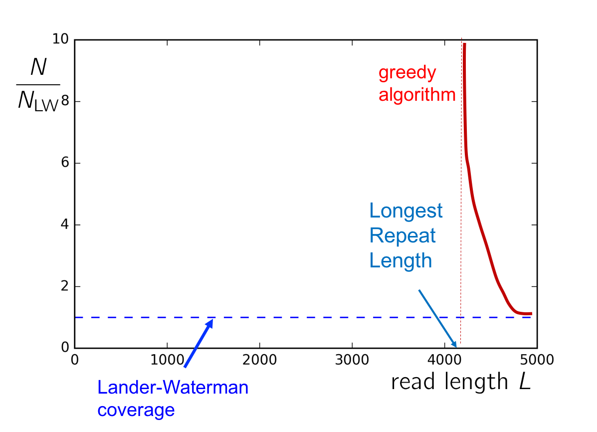
To gain a better sense of the conditions on \(c\) and \(L\) for successful assembly, consider the plot of \(c\) v. \(L\). If the read length is shorter than \(\ell_\text{max}\), the length of the longest repeat, then greedy cannot succeed. As \(L\) approaches \(\ell_\text{max}\) from the right, we need an asymptotically large amount of reads in order to cover this longest repeat with high probability. Additionally, if the coverage is too low (i.e. below the Lander-Waterman coverage), then successful assembly also cannot be achieved. The following figure summarizes when the greedy algorithm will succeed.
The probability that a repeat (assumed to have 2 copies) is not bridged is
\[\begin{align*} Pr(\text{repeat is not bridged}) = \left(1 - 2\frac{L-\ell-1}{G}\right)^N \end{align*}.\]We define \(Z\) to be the number of repeats not bridged. We then bound the probability that there exists one repeat not bridged using Markov’s inequality, just like in the coverage analysis:
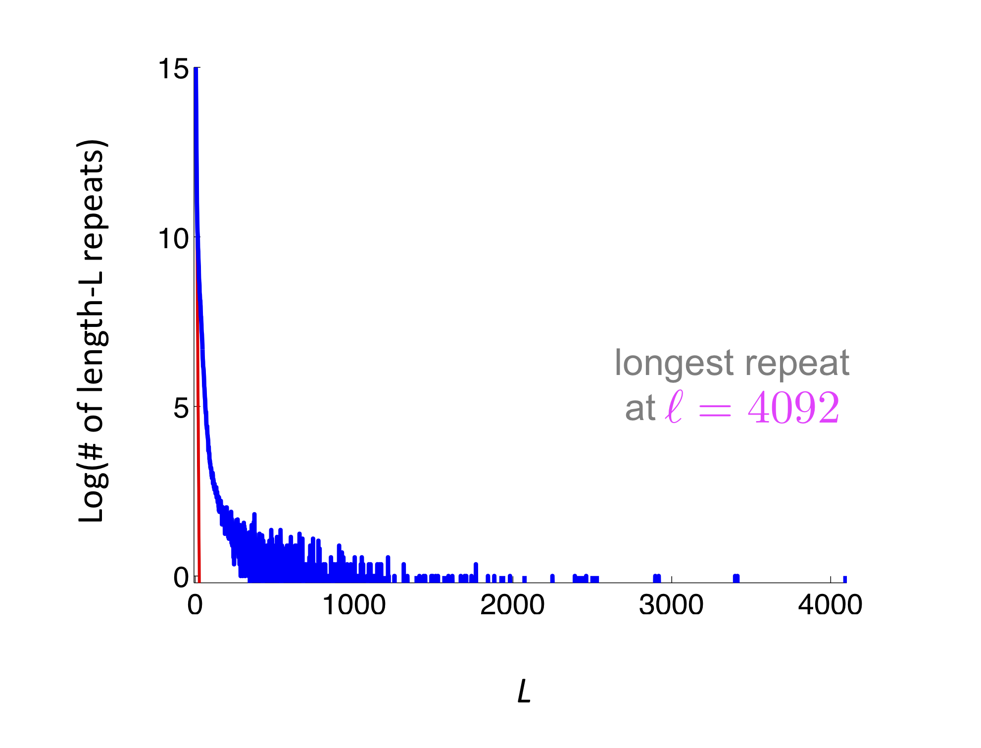
\[P(Z \ge 1) \le E[Z] = \sum_i \left(1 - 2\frac{L-\ell_i-1}{G}\right)^N\]where \(\ell_i\) is the length of the \(i\)th repeat and the summation is over all repeats. It can be seen that this bound depends only on the repeat distribution on the genome. We don’t care what the actual location of the repeat is. We show an example below where we have several short repeats. The red curve represents the repeat length distribution for a randomly shuffled genome. This figure shows that the human genome is far from a random sequence, and additionally it has quite a few high-length repeats (on the order of 1000s).
We also can ask: can we do better than the greedy algorithm? The Lander-Waterman statistic gives us a lower bound. We will derive a better algorithm in the next lecture.