Lecture 4: Base Calling for Next-Generation Sequencing
Lecture 4: Base Calling for Next-Generation Sequencing
Thursday 18 January 2018
scribed by Mark Nishimura and edited by the course staff
Topics
We last talked about Illumina reads, which are short (~100-200 bp long). For long read technologies, reads can reach the length of 10s of thousands of bp long. Today we will discuss the base calling problems associated with long-read technology.
Recap
Last time, we introduced a model for the errors introduced by the sequencing process as:
\[\mathbf{y}^A = Q\mathbf{s}^A + \mathbf{n}^A\]where \(\mathbf{s}^A\) is the 0-1 vector describing the locations of A’s in the DNA sequence, \(Q\) is a matrix representing errors in the read process (intersymbol interference), and \(\mathbf{n}\) is \(\mathcal{N}(0, \sigma^2)\) Gaussian noise. \(\mathbf{y}^A\) is the data we observe in the form of intensities of light captured from photos of the assay plate.
We considered models of the form:
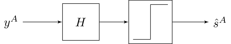
The step function here refers to symbol-by-symbol thresholding. The best \(H\) we came up last lecture with was from the MMSE formulation, but this strategy is not necessarily optimal because it does not use the fact that \(y \in \{0, 1\}.\)
Maximum Likelihood
We will now attempt to formulate the problem as a maximum likelihood (ML) problem (we will omit the \(A\) superscript to simplify the notation).
\[\text{argmax}_{\mathbf{s} \in \{0, 1\}^L} P(\mathbf{y} | \mathbf{s}) = \text{argmax}_{\mathbf{s} \in \{0, 1\}^L} \frac{1}{(2\pi)^{n/2} \sigma} \exp \left( \frac{-1}{2\sigma^2} \| \mathbf{y} - Q\mathbf{s} \|^2 \right) = \text{argmax}_{\mathbf{s} \in \{0, 1\}^L} \| \mathbf{y} - Q\mathbf{s} \|^2\]A brute-force approach would involve testing all \(2^L\) possible solutions, but this is intractable for even small \(L\). If we assume \(Q\) can take on any form, there is no easy way to solve this problem. Recall that for \(Q\), as we move away from the diagonal entries, the terms get smaller quickly. This is essentially because for a value of 1 at \(\mathbf{s}(i)\) to influence the reading of \(\mathbf{y}(j),\) there would need to be \(\left| i-j \right|\) independent failures in the sequencing process, each with its own (small) probability. Therefore we can approximate \(Q\) with a band-diagonal matrix. For now, we consider the case when only the main diagonal and the first lower diagonal \(Q\) (i.e. \(Q_{i,i-1}\), for \(i = 2...,L\)) are nonzero, with the rest assumed to be zero.
Given this band-diagonal assumption, the original equation \(\mathbf{y} = Q\mathbf{s} + \mathbf{n}\) becomes
\[\begin{align*} y(1) &:= Q_{11} s(1) + n(1) \\ y(2) &:= Q_{22} s(2) + Q_{21} s(1) + n(2) \\ y(3) &:= Q_{33} s(3) + Q_{32} s(2) + n(3) \\ & \vdots \end{align*}\]which can be summarized as
\[\min_{\mathbf{s}} \sum_{i = 2}^L [ y(i) - Q_{ii} s(i) - Q_{i, i-1} s(i-1) ]^2 + [y(1) - Q_{11}s(1)]^2.\]This objective can be minimized efficiently.
State Diagram
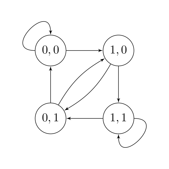
To solve this problem, we introduce the idea of a state. In the objective above, each term of the sum only depends on the value of \((s(i), s(i-1))\), and therefore
\[\text{state} = \begin{bmatrix} s(i-1) \\ s(i) \end{bmatrix}\]encapsulates all the information we need to produce a single (noisy) measurement \(y(i)\). Now, instead of a sequence of 0’s and 1’s \(s(1), s(2),\dots,s(L)\), we have a sequence of states \((s(1), s(2)), (s(2), s(3)), \dots\). In the first sequence, the value of \(s(i)\) does not depend on the value of $s(i-1)$; however in the second sequence, not all state transitions are allowed. They are summarized in the following diagram:
We can now view the optimization problem as a shortest path problem. \(\min_{\mathbf{s}} \sum_{i = 2}^L [c_i(s(i-1), s(i))]^2 + [y(1) - Q_{11}s(1)]^2.\)
where \(c_i(s(i), s(j)) = (y(i) - Q_{ii} s(i) - Q_{i,i-1}s(i-1)) \\) is the cost associated with transitioning states. Minimizing our objective corresponds to finding the minimum cost path (from left to right) through the trellis.
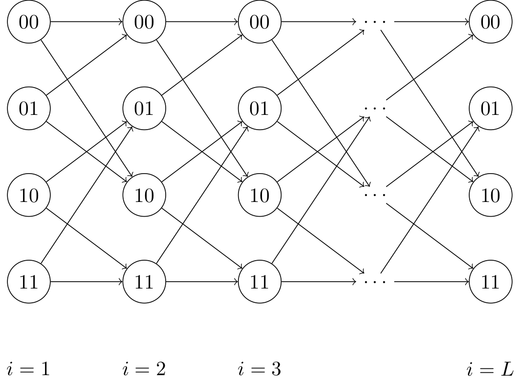
Each column represents a state \(s(i)\), and each state within that column is associated with a cost \(c_i(s(i), y(i))\) that is a function of our estimate of the state \(s(i)\) and our observation \(y(i)\). The minimum cost path is the path through the graph from left to right that minimizes the sum of the costs of the states through which it passes. This minimum cost path corresponds exactly to the sequence \(\mathbf{s}\) that minimizes our objective function.
We have \(L\) stages, and we can find the shortest path using the Viterbi algorithm (dynamic programming), which has runtime \(O(L2^b)\). \(b\) is the number of nonzero diagonals of our \(Q\) matrix (and hence, \(2^b\) is the number of states at each time step of the trellis)
Long Read Technologies
Recall that a major issue with short reads is the difficulty of resolving repeats, identical sequences within the reference genome. Technology that produce longer reads can help resolve this. We will discuss two strategies for long-read sequences pioneered by the two companies Oxford Nanopore and Pacific Biosciences. Both strategies perform single-molecule sequencing, which in contrast to second-generation sequencing technologies, does not require PCR.
Nanopore
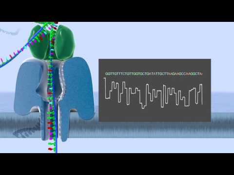
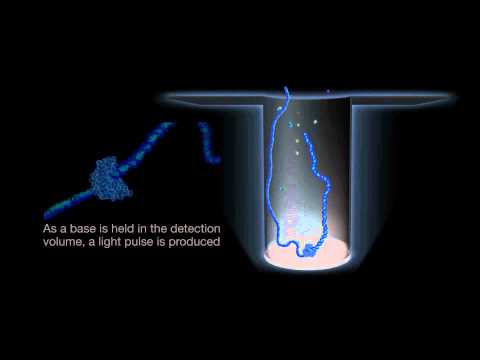
For nanopore technologies, each double-stranded DNA fragment is bound to a special enzyme. The enzyme binds to a nanopore, which is affixed to a substrate. The enzyme then unzips and advances the DNA through the nanopore one base at a time. A voltage across the nanopore produces a small electrical current, and the difference in resistances of different bases allows the DNA sequence to be determined based on this varying current signal (on the order of picoamperes or pA). Our length is no longer limited by the phasing or misalignment issue, but instead is limited by when our enzyme breaks down.
The error rate of Oxford Nanopore is relatively bad and on the order of 10-15% due to two major issues associated with this technology.
-
The size of a nanopore is bigger than a nucleotide, and therefore each electrical signal we measure is the signal aggregated from a few adjacent nucleotides (typically 3-6).
-
The DNA sequence does not move at a constant rate through the nanopore. Therefore when we segment the signal, we may skip bases or even backtrack. This leads to deletion and insertion errors, the major source of error for this technology.
A state-of-the-art approach (Mao et al. 2017) for performing base calling starts by sliding a length-4 window across our DNA sequence, resulting in length-4 sequences called contexts. Occasionally we may skip or backtrack. The dwell time is the time each window spends in the nanopore, or the time we read a particular current for. Level-finding is the process of of smoothening the noisy signal into discrete steps. Finally, we discretize the signal.
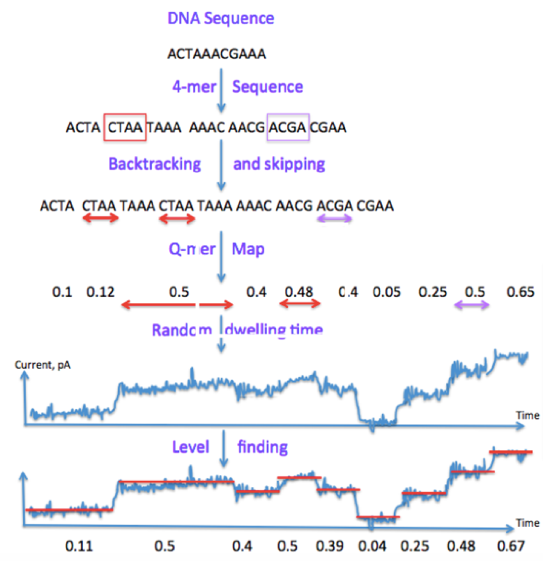
Leveraging our previous notation, we can summarize the process using the following block diagram:
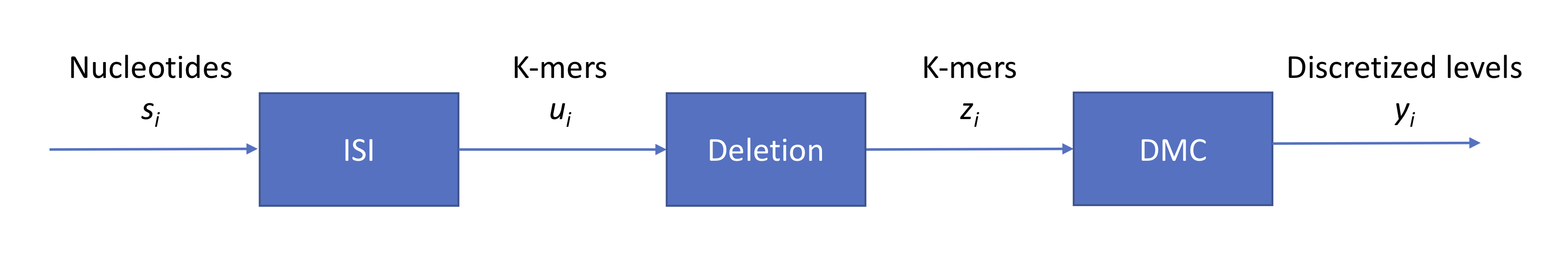
Note that \(s_i \in \{A, G, C, T\}\) while \(z_i \in \{A, G, C, T\}^4\). Now we have a base calling problem. Similarly to our approach for second-generation sequencing, we can again draw a state transition diagram. With 4-mers, we have \(2^8\) states. Given that we are in a certain state, how many states can we move to? Assuming that the probability of insertion or deletion is 0, then we can move to only one of 4 states.
In general, however, we can use our Viterbi approach from before. Each column in the trellis consists of \(2^8\) states. If the probability of skipping one or two bases is non-zero, then we simply add more edges to our trellis.
Pacific Biosciences
While Nanopore technology measures electrical current, PacBio technology measures colors emitted in microscopic wells called zero-mode waveguides (\(10^{-21}\) liters) during DNA synthesis. With tens of thousands of wells per so-called SMRT chip, each ZMW essentially allows us to read out color intensities at thousands of times stronger than the background signal. Like nanopore, the error rate of PacBio reads is also about 10-15%. The speed of the process of the single DNA molecule going through an enzyme causes randomness, resulting in the same insertion and deletion issues also associated with Nanopore technology.