Lecture 2: Basics of DNA & Sequencing by Synthesis
Lecture 2: Basics of DNA & Sequencing by Synthesis
Thursday 11 January 2018
Topics
In this lecture, we discuss how the sequencing process works for certain mainstream technologies. We first introduce some biological background before discussing two important sequencing technologies: Sanger (first generation sequencing technology) and Illumina (second generation sequencing technology). We want to gain some sense of how noise gets introduced into the process and how the technology has improved so drastically in the last two decades.
Basics of DNA
The human genome is the entire DNA sequence of a human individual. Human DNA comes in 23 pairs of chromosomes, and each pair contains one chromosome inherited from the mother and one inherited from the father, yielding 46 chromosomes total. 22 of the pairs are autosomal chromosomes, and the last pair are the sex chromosomes. Every cell in an organism contains the same exact genomic data living in the cell’s nucleus. In humans, the genome is 3 billion base pairs (bp) long. Different species have genomes of very different sizes. Bacterial genomes are a few million bp; most viral genomes are 10000s of bp; and certain plants have genomes of that are hundreds of billions of bp long. There are two types of cells: prokaryotic (no nucleus and found in organisms like bacteria) and eukaryotic (contains a nucleus and found in higher organisms like humans). While understanding the human genome is important, the techniques of this class are broadly applicable to other organisms.
DNA structure
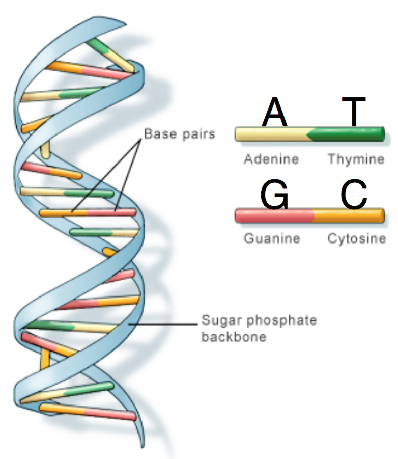
DNA is comprised of a sugar-phosphate backbone and four nucleotide bases: Adenine (A), Cytosine (C), Guanine (G), and Thymine (T). DNA is double-stranded and structured in a double-helix formation with pairs of nucleotides as “rungs” of the helix (hence the term “base pair”). Adenine always chemically binds with Thymine, and Cytosine always binds with Guanine. In other words, A is complementary to T, and similarly C is complementary to G. The A-T and C-G pairs are known as complementary pairs. The structure of DNA is shown below.
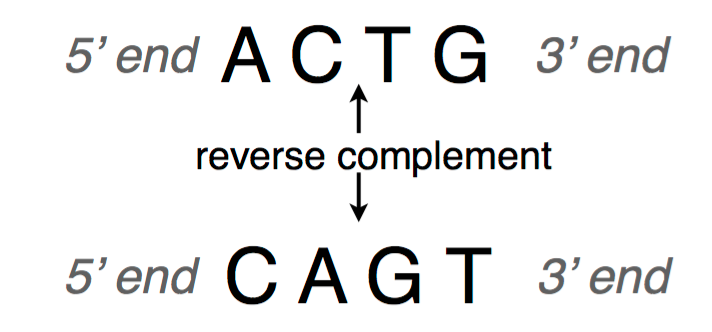
A DNA sequence is conventionally written in the 5’ end (head) to the 3’ end (tail) direction. When we write a DNA strand, we only write the letters representing the bases from one of the strands. The other strand, which is the reverse complement of the first strand, can be inferred because we know the complementary pairs. To get the reverse complement, we reverse the order of the nucleotides in the original string and then complement the nucleotides (i.e. interchange A with T and C with G). The figure below shows an example of a DNA fragment and its reverse complement strand.
DNA variation
Across humans, genomes are about 99.8% similar. Out of the 3 billion base pairs, individual genomes vary at 3-4 million base pair locations. These variations are captured in Single Nucleotide Polymorphisms (SNPs), though there are some large variations called Structural Variants (SVs). Because human genomes are so similar across individuals, we do no need to sequence the entire genome for an individual to observe their genome. Instead, we can sequence just the SNPs. Differences in the individual genomes arise due to two reasons:
- Random mutations, which occur during evolution because natural selection favors certain phenotypes. These arise mainly due to “errors” during the DNA replication process during cell division. Most of these mutations are deleterious, leading to phenotypic changes that are harmful and resulting in the death of the cell. Occasionally, natural selection favors certain mutations, and these are preserved in the population.
- Recombination, which occurs during reproduction in higher organisms like mammals. During recombination, the genetic material passed by the parent organisms to their child is a mixture of genetic material from the parents.
DNA replication
DNA lies at the foundation of cell replication. When a cell undergoes cell division, also known as mitosis, the DNA in its nucleus is replicated and through a series of steps shown in the figure below, one parent cell yields two identical daughter cells.
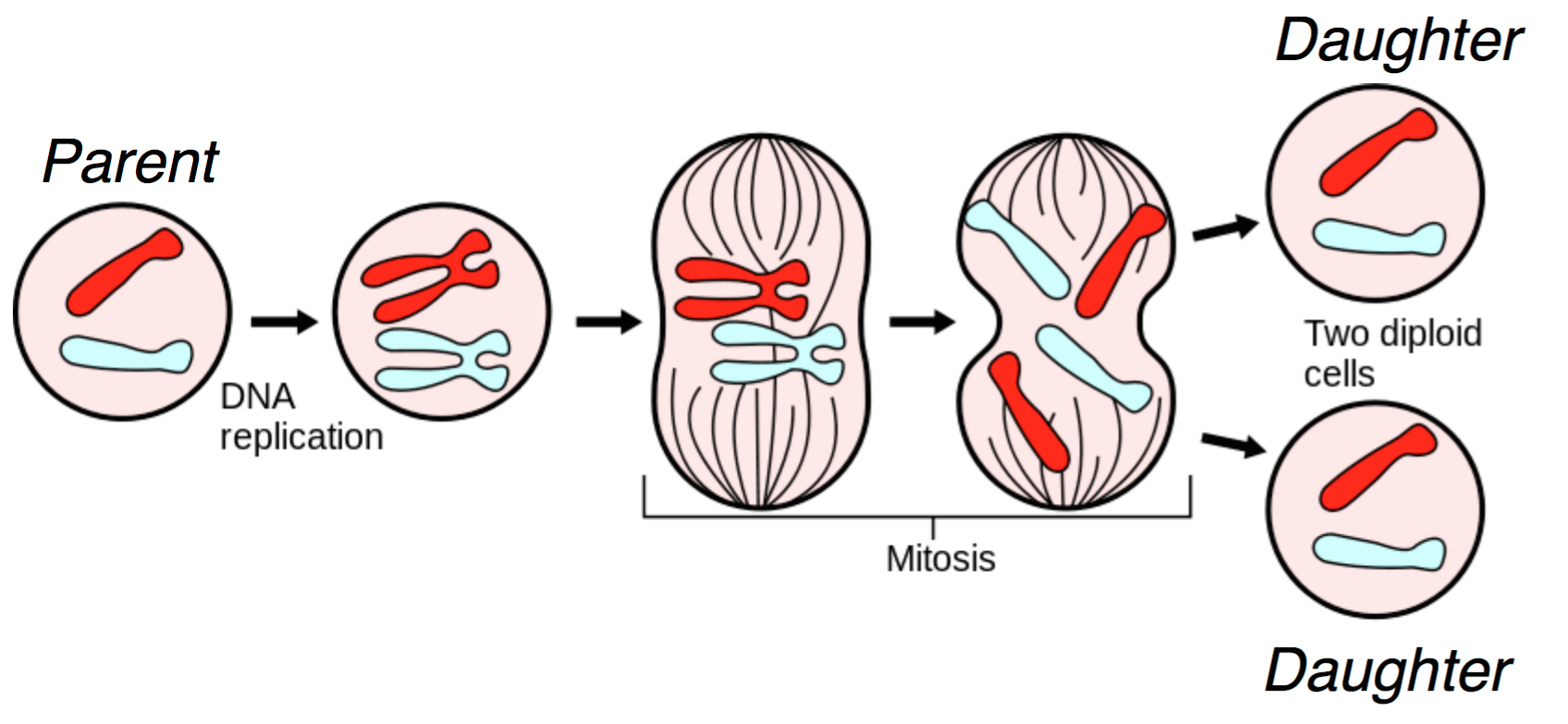
Several biomolecules are involved during mitosis, and we give a heavily simplified explanation of the mitotic process here. In the figure, we start with two chromosomes: red and blue. First, the DNA is replicated, resulting in the more familiar X-shaped chromosomes. Through a complex cascade of biomolecular signals and within-cell restructuring, the (now-replicated) chromosomes are lined up in the middle of the cell. For each chromosome, the halves are pulled apart, and each of the two daughter cells receives a copy of the original chromosome. This results in two daughter cells that are genetically identical to the original parent cell. For us, DNA duplication is the most important part of this diagram; this is the natural process we exploit in order to do sequencing.
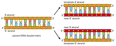
During DNA replication, the two strands of DNA are first unzipped, resulting in two single strands each acting as a template for replication. A short RNA primer is then attached to a specific site on the DNA; the bases in the primer are complementary to the bases in the site. An enzyme facilitates (or “catalyzes”) a chemical reaction, and DNA polymerase is the enzyme that catalyzes the complementary pairing of new nucleotides to the template DNA extending the bound primer. The nucleotides that DNA polymerase uses to extend a strand are called dNTPs (deoxynucleotide triphosphates). Biochemically, they are slightly different from the nucleotides in a way that makes them easier to work with during DNA replication. The dNTPs corresponding to A, C, G, and T are dATP, dCTP, dGTP, and dTTP, respectively. The DNA replication is illustrated below.
Sanger sequencing
The first technique used to get reads from DNA was a process called Sanger sequencing, which is based on the idea of sequencing by synthesis. Fred Sanger won his second Nobel prize for the invention of Sanger sequencing in 1977. Sanger sequencing was the main technology used to sequence genomic data until the mid 2000’s when the technology was replaced by second-generation generation sequencing technologies. The two sequencing techniques are related because they both use the sequencing by synthesis technique; however, second-generation sequencing massively parallelizes Sanger sequencing, resulting in a gain of roughly 6 orders of magnitude in terms of cost and speed.
We look at sequencing from a computational point of view, and we need to understand the technology a bit in order to motivate what we do. In the following, we try to answer the following 3 questions.
- How do we get 6 orders of magnitude improvement between Sanger sequencing and second-generation sequencing?
- How are errors introduced? All measurements have errors, and the reasons why these errors exist depend on the technology.
- Why is the read length limited? One of the biggest computational challenges of sequencing is that although the sequence of interest is very long (> 1M bp), the data we get is very short (~100 bp).
Sequencing by synthesis
Sequencing by synthesis takes advantage of the fact that DNA strands, which are normally in double-helix form, split apart for mitosis and each strand is copied. Sanger figured out a clever way of converting the sequencing problem into a problem of measuring mass.
We mentioned above that DNA polymerase naturally uses dNTPs to synthesize a new strand. The synthesis process occurs very quickly, making it hard to make any sort of measurement during synthesis. Sanger overcame this problem by figuring out a way to terminate synthesis using a modified version of dNTPs called ddNTPs (dideoxynucleotide triphosphates). DNA polymerase can attach a ddNTP to the sequence just like with dNTPs, but it cannot attach anything to the ddNTP. In other words, the attachment of a ddNTP halts the replication of the DNA molecule.
We will denote ddNTPs corresponding to A, C, G, and T as A*, C*, G*, and T*. By introducing a small amount of one type of ddNTP into the experiment (e.g. T*), when the reactions finish, we are left with: 1. small percentages of strands containing T*s at locations corresponding to A’s in the template, and 2. a large fraction of strands containing only normal dNTPs. This procedure is known as the chain termination method. We now describe Sanger’s sequencing procedure created in 1977:
-
We first replicate the sequence using a technique called polymerase chain reaction (PCR), which also takes advantage of DNA replication to exponentially increase the amount of DNA. For our purposes, we will assume that after running \(N\) cycles of PCR, we obtain \(2^N\) times the original amount of the molecule. PCR dramatically increases the amount of biological material.
-
We break apart the two strands by heating up the sample. One of the single strands will be used as the template strand or the strand to which new bases will be attached.
-
We add a template strand of DNA to a test tube along with free-floating dNTPs and a few modified ddNTPs (1% of the nucleotides). All ddNTPs are of the same type. We also add a primer or a short sequence that attaches to the beginning of the strand of interest and starts the whole replication process.
-
We filter out sequences that end in ddNTPs using a technique called gel electrophoresis. This method exploits the fact that the DNA molecule has a charge. By putting the DNA sample in a gel and inducing an electric field over the gel, we can separate strands of different masses (larger strands move slower).
-
We measure the mass of isolated strands. This can be done by either radioactively labeling nucleotides and measuring the level or radioactivity or by adding florescent tags to the nucleotides and measuring the strength of the light emitted (i.e. take a picture).
The figure below illustrates a simple example showing the process of Sanger sequencing.
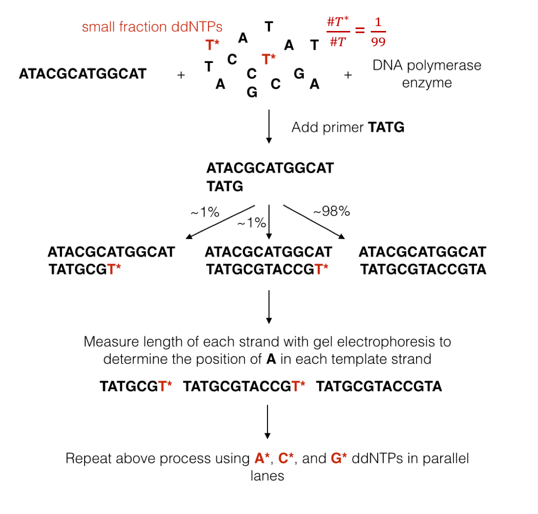
In another example, suppose we obtain the following data for each of the four nucleotides. Each number represents how far along the gel a fragment ending with a certain nucleotide traveled.
| A | C | G | T |
|---|---|---|---|
| 30.0 | 48.2 | 56.7 | 86.3 |
| 61.3 | 99.3 | ||
| 74.4 |
Merging these 4 sorted lists gives us the underlying sequence. In the example we get
30.0 - A
48.2 - C
56.7 - G
61.3 - A
74.4 - A
86.3 - T
99.3 - C
giving us the sequence to be ACGAATC.
Limitations of Sanger sequencing
Sanger sequencing works for sequences below roughly 700 bp in length. This read limitation stems from the fact that as the length \(L\) of a sequence increases, distinguishing between the mass of a length \(L\) sequence and the mass of a length \(L+1\) sequence becomes increasingly harder. To see this, note that a tolerance of 0.1% in measurement would make it impossible to distinguish a sequence of length 1000 from one of length 1001 even if all bases had the same molecular weight. Such errors in measuring mass are also a reason for errors in Sanger sequencing, though the error rate is around 0.001%.
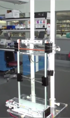
Additionally, Sanger sequencing is slow (low-throughput) because the mass measuring process is time consuming. Sanger sequencing allowed scientists to sequence around 3000 bases per week. One of the main reasons that the procedure is slow is because it requires measuring the mass of many molecules, a costly process. The equipment used for Sanger sequencing is shown below.
Illumina sequencing
Second-generation sequencing, pioneered by Illumina, makes a few modifications to the Sanger process shown above. The sequencing procedure also massively parallelizes the process, dramatically increasing the throughput while decreasing the price.
Illumina achieves parallelization by running several synthesis experiments at once. Each of many template strands is anchored on a chip, and only ddNTPs with florescent tags are available during the synthesis procedure (no dNTPs). Each type of ddNTP is tagged such that it emits a different wavelength or color. Since ddNTPs halt synthesis, the synthesis of new strands are synced. All new strands are the same length at the end of each synthesis cycle, at which point a picture of the chip is taken. These pictures are then analyzed by “base caller” software to identify (or “call”) the complementary nucleotides. Base calling will be discussed in greater detail next lecture. To override the chain termination, Illumina sequencing uses reversible termination. The sequencing process introduces an enzyme which can turn a ddNTP into a regular dNTP after it has bound, allowing the synthesis reactions to continue instead of being permanently halted. For the MiSeq, a single cycle takes about 6 minutes.
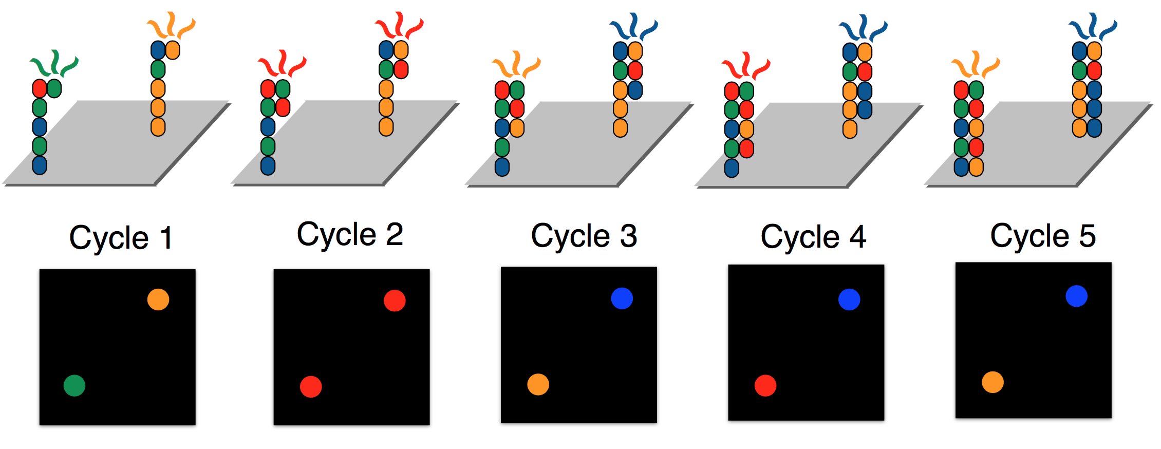
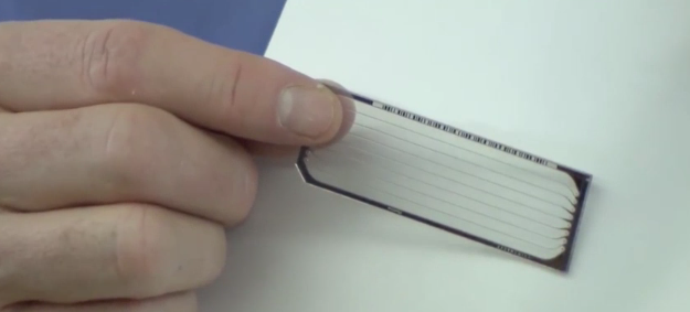
In order to guarantee that enough light is emitted such that ddNTP signals are detectable, each of the template strands are cloned, resulting in clusters of the same strand being synthesized in unison. Because of reversible termination, Illumina sequencing removes the need to measure masses. In contrast to the gel electrophoresis procedure required for Sanger sequencing above, the figure below shows a glass slide used during Illumina sequencing. Illumina sequencing can sequence billions of template strands simultaneously, which greatly increases the throughput.
Errors in Illumina sequencing arise due to time steps where no ddNTP attaches to some sequence and hence the same base is read twice. Additionally, dNTPs still exist in solution, and therefore occasionally a dNTP rather than a ddNTP may be attached to a strand being synthesized. The DNA polymerase then continues synthesis until it adds a different ddNTP. For this reason, although all strands within each cluster are identical, the photograph may be noisy.
-
Slides on Biological Background : Borrowed from Ben Langmead’s slides
-
Slides on Sequencing by Synthesis : Borrowed from Ben Langmead’s slides
-
Ben Langmead’s animation showing Sequencing by Synthesis
-
The Sanger sequencing figure was made by Claire Margolis. The DNA replication figure is taken from Alberts B, Johnson A, Lewis J, et al, Molecular Biology of the Cell. 4th edition. The rest are taken from Ben Langmead’s notes.