Lecture 16: Single Cell RNA-Seq - Introduction
Lecture 16: Single Cell RNA-Seq - Introduction
Thursday 1 March 2018
scribed by Po-Hsuan Wei and edited by the course staff
Topics
Motivation
In previous lectures, we discussed bulk RNA-seq, which at a high level can be described by: sample → cell lysis → reverse transcription → amplification → sequencing → read-alignment → quantification → transcript population.
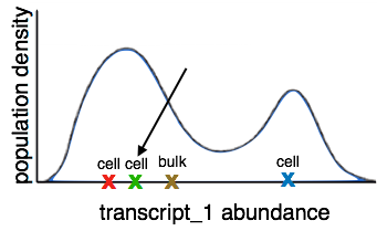
Since multiple cells were lysed together, the transcript abundance we get at the final step is a population average of all cells in the sample. This prevents us from differentiating between changes in regulation within cells and compostion of the sample of cells. We also lose cell differentiation information as the cells in a sample have various differentiation rates and are therefore in different stages of differentiation.
Sequencing platforms
Tang et al. (2009) obtained a single-cell transcript abundance by isolating the cell before lysis. The abundance data from one cell, however, is not sufficient to represent the transcriptome distribution. Since multiple single-cell sequencing is necessary, the time-consuming and expensive procedure carried out by Tang et al. was replaced by platforms that parallelize the preparation process up to the sequencing step. Fluidigm C1 speeds up the isolation process by trapping and releasing single cells into individual microfluidic channels whereas Drop-Seq uses droplets and “tags” to allow for joint downstream processing.
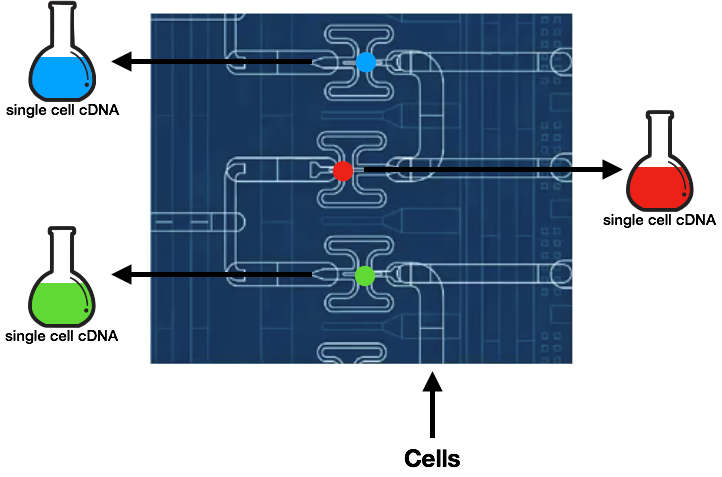
Fluidigm C1
The microfluidic chip traps a cell per capture site, and the cells are subsequently flushed to obtain single cell samples per pipe. The cells then undergo cell lysis, reverse transcription, and amplification within its own chamber. The resulting products are then ready to be sequenced.
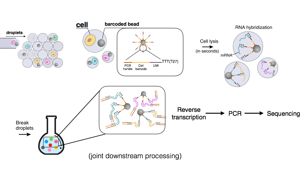
Drop-Seq
Drop-Seq uses microfluidics to compartmentalize a barcoded bead, a cell, and lysis buffer. Each bead has millions of primers attached, and each primer consists of a PCR handle, a cell barcode, a UMI (unique molecular identifier), and a long tail of T nucleotides. The cells are lysed within each droplet, and their mRNAs hybrize to the long T-tail on the primers. Subsequently, the droplets are broken, and all mRNAs are reverse transcribed and amplified with PCR.
The sequencing step is done using paired-end reads where the first read of the pair always coincides with the cell (barcode + UMI) part of the primer.
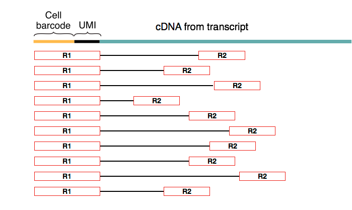
Drop-Seq aims to trace molecules back to each cell, and this is achieved by using a 12bp cell barcode to distinguish different cells and an 8bp UMI to differentiate molecules within the same cell. UMIs are particularly useful for removing the sequence-specific biases associated with PCR.
Since expression information is encoded in the cDNA, we don’t need to worry about collision of UMIs between different transcripts in the same cell. Still, we can calculate the expected number of collisions:
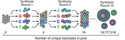
\[\begin{align*} N & = \text{# of molecules in the same cell} \approx 100000 \\ B & = \text{# of distinct UMIS } = 4^8 \approx 64000 \\ X_i & = \text{the UMI of the } i \text{th cell} \\ P(X_i = k, X_j=k) & = 1/B^2 \\ P(X_i = X_j) & = 1/B \\ E[\text{# of collisions}] & = N(N-1)/2B \approx 3.2 * 10^{14} \end{align*}\]One method for generating barcodes is known as splitting and pooling. In this process, we start with a collection of beads and four “buckets” of nucleotides, one for each nucleotide. We split the beads randomly into four parts, dip them into the corresponding buckets, re-mix them, and repeat. This will result in several random barcodes.
Computational workflow of Drop-Seq
After obtaining reads consisting of cell barcode, UMI and cDNA, we can estimate the transcript abundances. We first group reads by cell barcode before aligning cDNA reads and counting unique molecules per cell per gene using the UMIs.
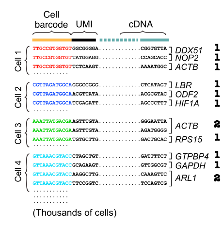
The final output is a gene expression table, with columns representing cells and rows representing genes. There are 2 major sources of errors:
- Errors during sequencing and synthesis of barcodes
- A droplet capturing more than one cell
For the first kind of error, since the barcode is short, we can simply filter out the erroneous barcodes by choosing the ones with many read counts.
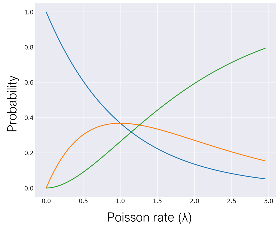
For the second kind of error, we can model the cell capture success rate using a Poisson process with some Poisson rate \(\lambda\), which we tune using the concentration of cells. With a high Poisson rate (and therefore a high cell concentration), we would obtain more multiplets, less singlets, and less empty droplets. If 2 cells with similar mRNA counts get trapped together, then the read count effectively doubles for reads with the same cell barcode. If the 2 cells in a doublet have very different mRNA counts, then the transcript support would be longer than in either of the individual cells.
Parting thoughts
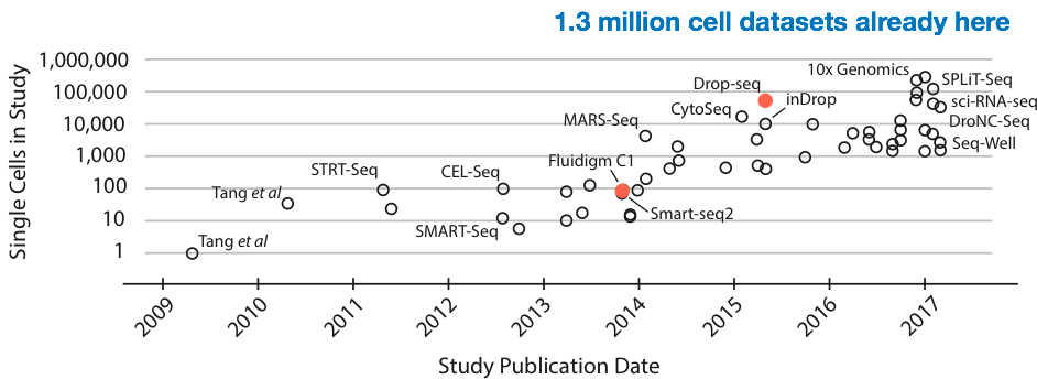
While sequencing cost is going down quickly (faster than Moore’s law), there is also a different curve of interest that’s been growing exponentially: the size of single-cell RNA-Seq experiments (in terms of number of cells). Most recently, 1.3 million cells have been sequenced by 10X genomics. At approximately $0.00001 per read, this would cost on the order of half a million dollars. Sequencing cost is becoming the bottleneck again.