Lecture 14 - RNA-seq - Quantification and the EM Algorithm Part 2

Lecture 14 - RNA-seq - Quantification and the EM Algorithm Part 2

Tuesday 20 February 2018

scribed by Mira Moufarrej and edited by the course staff

Topics

1. Estimating RNA Abundance
2. Hard vs Soft EM
3. EM as alternative maximization
4. Pseudo-alignment

Estimating RNA Abundance

When we sequence RNA, we would like to quantify the abundances of distinct transcripts. As we have seen previously, NGS yields short reads that can map back to multiple transcripts. For instance, if we have a read composed of an exon \(B\), and we have two transcripts where transcript 1 is \(ABC\) and transcript 2 is \(BCD\), the read maps to both transcripts 1 and 2. This is known as the multiple mapping problem.

Here, we want to infer each transcript’s abundance based on the read data. Let \(Y\) be the data (reads). Let \(\rho\) be a vector of unknown abundances for each transcript, which we want to estimate. Using maximum likelihood (ML), we can infer the most likely estimate of \(\rho\) based on the data \(Y\). Using the ML formula, we would get the following,

However, this formula is computationally intractable. We would like to infer \(\rho\) based on the data, but \(Y\) inherently depends on \(\rho\). Therefore, we try to solve an easier problem.

Let \(Z = (Z_{ik})\) be a hidden variable such that \(Z_{ik} = 1\) if read \(i\) comes from transcript \(k\). If we knew \(Z\), we will see that ML inference becomes a lot easier, and we could write the ML problem as:

Using the chain rule to expand this joint probability, we get that:

Since \(P(Y|Z)\) has no dependence on \(\rho\), we can treat it as a constant and rewrite the expression above as maximizing only the second term:

But what is \(P(Z;\rho)\) and is it tractable? Assuming all transcripts are the same length, we can rewrite \(P(Z;\rho)\) as follows:

where \(Z_{ik}\) is an indicator function that equals 1 when read \(i\) comes from transcript \(k\). If transcripts were of different lengths, we would scale by length. Taking the log of the expression for \(P(Z;\rho)\), we get the following:

Notice that in this expression, each transcript contributes one log term and \(\sum_{i=1}^N Z_{ik}\) is the number of reads sampled from transcript \(k\). This expression is computationally tractable. Therefore if we knew \(Z\), we would be able to solve for \(\hat{\rho}_{ML}\). This is the same as the estimation problem for when all reads are uniquely mapped. By revealing \(Z\), one converts the multiple mapping problem to a unique mapping problem.

But because we don’t know \(Z\), we can use EM to maximize both \(\rho\) and \(Z\) iteratively. Why does this work? Notice that in the original ML formula, we had that:

This is essentially equivalent to marginalizing \(Z\) out of the sum (computationally intractable), which can be approximated as maximizing over the joint probability of \(Y\) and \(Z_{MAP}\) where \(Z_{MAP}\) is the maximum a posteriori estimate of \(Z\) given \(Y\).

However, this is a chicken and egg problem since computing \(Z_{MAP}\) requires knowledge of \(\rho\).

Hard vs Soft EM

We start with some initial value for \(\rho\) called \(\rho^{(m)}\). Given these values of \(\rho\), we find the values of \(Z\) that maximizes the probability in the objective (maximum a posteriori).

This type of EM is called hard EM. This inference process is attempting to estimate the hidden variable (the transcript a read comes from) for each read. If a read could potentially come from, say, 3 different transcripts, we pick the transcript with maximum probability. In hard EM, we make a hard decision on the hidden variable at each iteration. The drawback with this approach is that we do know for sure that a read comes from the max-probability transcript, and it may feel a bit aggressive.

Alternatively, instead of making a hard decision, we can instead average over the posterior distribution before continuing the inference step, resulting in a soft version. This results in the EM algorithm we discussed in the last lecture.

EM as alternative maximization

So far, we have attempted to justify EM from an intuitive point of view. We still have a problem, however, as the current method still seems somewhat heuristic. How do we know if this algorithm actually gives us the ML solution? To understand the connection of EM with maximum likelihood, we can define

where \(D(P_1 \| P_2)\) is the Kullback-Leibler divergence (KL-divergence):

and intuitively measures the similarity between the two distributions \(P_1\) and \(P_2\). Note that if we maximize over \(Q_Z\), we will get \(D(Q_Z \| P(Z|Y; \rho)) = 0\) , resulting in \(F(Q_Z, \rho) = \log P(Y; \rho)\). Therefore

This gives us an alternate maximization procedure:

1. Fix \(\rho\), max over \(Q_Z\)
2. Fix \(Q_Z\), max over \(\rho\)

and the problem now becomes: is this procedure easy to do? We see that

For step 2, we have \(Q_Z\) fixed, and therefore maximizing \(F(Q_Z, \rho)\) is just maximizing this final expectation over \(\rho\). In other words, step 2 is equivalent to

for fixed \(Q\). We see that the two steps of the alternate maximization procedure correspond exactly to the E and M steps in the EM algorithm. Technically, the E step here also requires maximization, and therefore perhaps MM is a more suitable name (see here).

As a note about existing software, Cufflinks and RSEM are both early tools that implement this EM approach.

Pseudo-alignment

Taking a step back, recall that the RNA-Seq problem involves determining which of several transcripts in a transcriptome a read comes from. The EM step is actually computationally cheap compared to aligning 100M reads, and therefore alignment is the computational bottleneck. But for the purposes of EM, do we really need alignment?

The fundamental problem here is the ML problem

where we have a data matrix

with \(Y_{ij} = 1\) if read \(i\) aligns to transcript \(j\).

Starting in about 2013, people started asking if we could recover \(Y\) without performing full alignment. For each read \(r\), we need to compute \(S\) of transcripts from which \(r\) can come. Recall that for aligning reads to a long genome, we broke each read up into \(k\)-mers. For each \(k\)-mer, we could quickly find where it maps to using a hash table. In other words, we indexed the genome first by building a hash table where \(k\)-mers are keys. This is much faster than doing full-scale alignment. We exploit the fact that even in the event of errors, a shorter \(k\)-mer sequence is less likely to have errors, and therefore we have a reasonable chance of getting exact mappings of the \(k\)-mers.

Similarly, we can also index the transcriptome by building a hash tables of all the \(k\)-mers. As an aside, we cannot choose even values for \(k\) (see assignment 3). Each 31-mer, for instance, will map to set of transcripts that \(k\)-mer can come from. Note that we do not concern ourselves too much with the computational cost associated with building this table as we only need to do it once (and thus the cost is amortised). The procedure will look something like

1. Build index (hash table)
2. Quantification

For each read, we will attempt to find the transcripts that the read belongs to. For each \(k\)-mer in the read, we obtain a set of transcripts (a few \(k\)-mers will be erroneous, but they will likely not map to any entry in the table). To find the unique set of transcripts that all the \(k\)-mers can come from, we can just take an intersection of the sets. Therefore the “alignment” step here consists of

1. Break read into \(k\)-mers
2. For each \(k\)-mer, get the set of transcripts that \(k\)-mer maps to
3. Take intersection of all transcript sets

Note that since we are not tracking positional information (yet), these transcript sets are a bit bigger than they could be. To incorporate the positional information, we can use a data structure similar to a \(k\)-mer overlap graph:

Pseudo-alignment figure from kallisto paper.

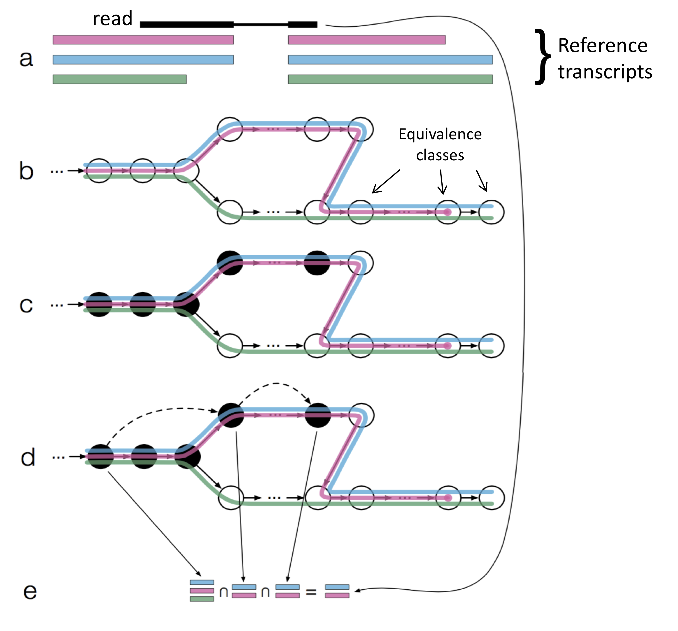
This strategy, known as pseudo-alignment, is used by kallisto and Salmon.