Lecture 12: RNA-seq - A Counting Problem
Lecture 12: RNA-seq - A Counting Problem
Thursday 15 February 2018
scribed by Logan Spear and edited by the course staff
Topics
In the previous lecture, we introduced RNA-seq and the quantification problem. In this lecture, we dive deeper into this problem – in the case when we know the RNA transcripts beforehand – and examine how we can solve it optimally under some simplicity assumptions.
- RNA-Seq quantification
- Improved approach: Iterative estimation refinement
- Evaluating the EM algorithm
RNA-Seq quantification
As discussed in the last lecture, the RNA-seq data consists of multiple reads sampled from the various RNA transcripts in a given tissue (after the reverse transcription of RNA to cDNA). We assume that these reads are short in comparison to the RNA transcripts.
We also assume that we know the list of all possible RNA transcripts \(t_1,t_2, \dots,t_K\) beforehand. Every read \(R_i,i=1,2,\dots,N \ \\) is mapped (using alignment) to (possibly multiple) transcripts. Our goal is to estimate the abundance of each transcript \(\rho_1, \rho_2,...,\rho_K, \\) where \(\rho_k \in [0,1], \ k \in \{1,2, \cdots, K \} \ \\) denotes the fraction of \(t_k\) among all transcripts.
Additionally, we make the following assumptions for the sake of simplicity:
- All transcripts have equal length \(\ell\). It is fairly straightforward to extend our analysis to transcripts of unequal length.
- Each read has the same length \(L\).
- Each read can come from at most one location on each transcript. This is a reasonable assumption, since different exons rarely contain common subsequences.
- The reads come from uniformly sampling all the transcripts. This is a relatively mild assumption we have made before to ease our analysis, even though it is not entirely accurate.
A naive approach
At the end of the last lecture, we discussed how we can simply count the number of reads that align to each transcript. We consider the following example where we have two transcripts \(t_1, t_2\) sharing a common exon B:
We consider two types of reads:
- uniquely mapped reads (e.g. reads that align to either exon A or exon C)
- multiply mapped reads (e.g. reads that align to exon B)
The difficulty of the above counting problem lies in the existence of the latter type of read. The simplest strategy for handling these types of reads is to just throw them away and work with only uniquely mapped reads. We see immediately that this approach fails if all the reads for a transcript comes from only exon B.
A less naive approach to deal with these reads would be to split them, i.e. assign a fractional count to each transcript a read maps to. We can split a multimapped read equally among all transcripts it is mapped to. For our example above, if a read maps to exon B, then each transcript gets a count of \(\frac{1}{2}\). Finally, our estimate of the abundance of \(t_k\) with total count \(N_k\) is
\[\hat{\rho}_k=\frac{N_k}{N}\]While naive read splitting sounds reasonable, it can fail spectacularly as well. Assume our ground truth is that \(\rho_1=1\) and \(\rho_2=0\). As a result, some of our \(N=20\) reads come from exon A and some come from exon B. Let’s assume that half of the reads come from each exon (even though the figure above does not depict the two exons as of equal length).
All the reads coming from exon A map uniquely to \(t_1\) and thus they contribute a total of \(\frac{20}{2}=10\) to the count \(N_1\) of \(t_1\). All \(\frac{20}{2}=10\) reads coming from exon B map to both transcripts and according to the naive algorithm above, each of them contributes \(\frac{1}{2}\) to each of the counts \(N_1, N_2.\) As a result, our estimate is that
\[\hat{\rho}_1=\frac{10+10*0.5}{20}=0.75,\] \[\hat{\rho}_2=\frac{10*0.5}{20}=0.25,\]which is clearly wrong.
Improved approach: Iterative estimation refinement
Since the naive algorithm fails, we need to come up with a better solution. We note that despite the failure, we came closer to the truth (in comparison to a random guess of equal abundances). Is there a way to leverage the information we gained? For example, what if we were to use our newly obtained estimate of abundances to re-split the multiply-mapped reads with weights proportional to the relative abundances of the two transcripts? In the above example, this would mean that
\[\hat{\rho}_1^{(2)}=\frac{10+10 \times 0.75}{20}=0.875,\] \[\hat{\rho}_2^{(2)}=\frac{10+10 \times 0.25}{20}=0.125,\]which is closer to the truth.
But now, we can simply repeat the process using the updated estimate of the abundances. It is easy to see that at each step, \(\hat{\rho}_2^{(m)}\) will be halved and hence, this process converges to the ground truth at an exponential rate.
This seems promising. So, let’s formulate this algorithm more generally.
General Algorithm for Sequences of Same Length
-
Since we know nothing about the abundances to begin with, our initial estimate is uniform. That is
\[\hat{\rho}_k^{(1)}=\frac{1}{K},k=1,2,…,K\] -
For step \(m=1,2,...\) repeat:
- For \(i=1,2,..,N\) let read \(R_i\) map to to a set \(S_i\) of transcripts, denoted by \(R_i \to S_i\).
Then, split \(R_i\) into fractional counts for each transcript \(k \in S_i\), equal to the relative abundances of the transcripts in \(S_i\),
as follows:
\(f_{ik}^{(m)}=\begin{cases} \frac{\rho_k^{(m)}}{\sum_{j \in S_i}{\rho_j^{(m)}}} &\text{if }k \in S_i \\ 0 & \text{otherwise} \end{cases}\) - The updated estimate is, obviously,
\(\hat{\rho}_k^{(m+1)}=\frac{1}{N}\sum_{i=1}^{N}{f_{ik}^{(m)}}\)
- For \(i=1,2,..,N\) let read \(R_i\) map to to a set \(S_i\) of transcripts, denoted by \(R_i \to S_i\).
Then, split \(R_i\) into fractional counts for each transcript \(k \in S_i\), equal to the relative abundances of the transcripts in \(S_i\),
as follows:
Let there exist two transcripts \(t_1\) and \(t_2\) of abundances \(\rho_1 =1 \\) and \(\rho_2 =0 \\) as shown below where there are three exons A, B and C all of equal lengths.
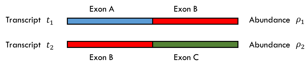
The initial read assignment will be
- read from Exon A \(\longrightarrow\\) +1 to \(t_1\), +0 to \(t_2\)
- read from Exon B \(\longrightarrow\\) +0.5 to \(t_1\), +0.5 to \(t_2\)
- read from Exon C \(\longrightarrow\\) +0 to \(t_1\), +1 to \(t_2\)
Assume we collect 40 reads: 20 reads from exon A and 20 from exon B. With this model, we would assign \(20 + 10(0.5) = 30\\) reads to \(t_1\) and \(0 + 20(0.5) = 10\\) to \(t_2\), which results in \(\hat{\rho_1} = \frac{30}{40} = 0.75\) and \(\hat{\rho_2} = \frac{10}{40} = 0.25\). Our estimates, however, are way off as 0.25 is much more than 0.
The algorithm gives us a way to improve our estimates. We can use our new \(\hat{\rho}\) values to determine what weights we should use when assigning the values from the multi-mapped reads. Thus, in this case, we can change the weight assignment for reads from exon B to
- read from Exon B \(\longrightarrow\\) +0.75 to \(t_1\), +0.25 to \(t_2\)
The weights are equal to the \(\hat{\rho}\) values in this case because the reads are of equal length. Now, we can recompute our estimates of \(\hat{\rho_1}\) and \(\hat{\rho_2}\) according to this new distribution of credit. Thus in the second iteration of the algorithm, we have that the count for \(t_1 = 20 + 20(0.75) = 35\\) so \(\hat{\rho_1} = 0.875\\). Similarly, the count for \(t_2 = 0 + 20(0.25) = 5\\) so \(\hat{\rho_2} = 0.125\\).
In this case, each iteration is taking us half the remaining distance to the ground truth (1 and 0). If you repeat this process, it will converge to the ground truth.
General Algorithm for Sequences of Different Lengths
Now we assume that we have \(K\) transcripts \(t_1, t_2, \cdots, t_k\\) of known lengths \(\ell_1, \ell_2, \dots, \ell_k\\). Let \(\rho_1, \dots , \rho_k\\) be the abundances of each of the transcripts. We define \(\alpha_i\\) as the normalized abundance of transcript \(t_i\\), which is the expected fraction of reads one would expect from transcript \(t_i\). More concretely
\[\alpha_k = \frac{\rho_k \ell_k} {\sum_{j=1}^K\rho_j \ell_j},\ \ k=1,2,…,K\]
\[\rho_k = \frac{\frac{\alpha_k}{\ell_k}} {\sum_{j=1}^K \frac{\alpha_j}{\ell_j}},\ \ k=1,2,…,K\]
We now define the EM algorithm as before estimating \(\alpha_i\) and inferring \(\rho_i\) from them.
-
Since we know nothing about the abundances to begin with, our initial estimate is uniform. That is
\[\hat{\rho}_k^{(1)}=\frac{1}{K},k=1,2,…,K\] -
For step \(m=1,2,...\) repeat:
- For \(i=1,2,..,N\) let read \(R_i\) map to to a set \(S_i\) of transcripts,
denoted by \(R_i \to S_i\).
Then, split \(R_i\) into fractional
counts for each transcript \(k \in S_i\), equal to the
relative abundances of the transcripts in \(S_i\),
as follows:
\(f_{ik}^{(m)}=\begin{cases} \frac{\rho_k^{(m)}}{\sum_{j \in S_i}{\rho_j^{(m)}}} &\text{if }k \in S_i \\ 0 & \text{otherwise} \end{cases}\) - The updated estimate of \(\alpha_i\) is, obviously,
\(\hat{\alpha}_k^{(m+1)}=\frac{1}{N}\sum_{i=1}^{N}{f_{ik}^{(m)}}\) - The updated estimate of \(\rho_i\) is then \(\hat{\rho}_k^{(m+1)}=\frac{\frac{\alpha_k^{(m+1)}}{\ell_k}} {\sum_{j=1}^K \frac{\alpha_j^{(m+1)}}{\ell_j}}\)
- For \(i=1,2,..,N\) let read \(R_i\) map to to a set \(S_i\) of transcripts,
denoted by \(R_i \to S_i\).
Then, split \(R_i\) into fractional
counts for each transcript \(k \in S_i\), equal to the
relative abundances of the transcripts in \(S_i\),
as follows:
Assume we have two transcripts \(t_1\) and \(t_2\) of abundances \(\rho_1 =0.75 \\) and \(\rho_2 =0.25 \\) as shown below where there are two exons A and B of equal lengths. Note that \(\ell_1 = 2 \ell_2\) in the example.
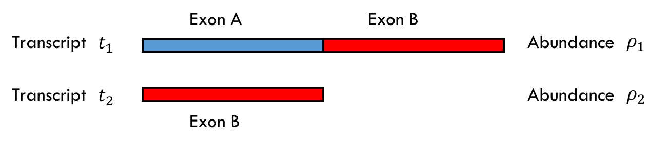
Before we go further, note the sampling model is not as straightforward as in the first example. Because the transcripts are different lengths we must consider their lengths when considering the probability that a read comes from that transcript. You can imagine the read sampling model as appending together all of the transcripts according to their abundance and then randomly taking a read from that single, long sequence. In this case, for \(\rho_1=0.75\) and \(\rho_2 = 0.25\), you can imagine first appending three copies of \(t_1\) and one copy of \(t_2\) together, and then sampling a read from this long sequence.
If we collect 70 reads, we can expect 30 to come from exon A in \(t_1\), 30 to come from exon B in \(t_1\), and 10 to come from \(t_2\). For simplicity assume we see exactly that.
Now that the transcripts are different lengths, the EM algorithm will involve an extra, intermediate step. To account for this, we will be introducing a new set of intermediate variables: \(\alpha_1\) and \(\alpha_2\) are the fraction of reads assigned to transcript 1 and transcript 2 according to the \(\rho\) values for the given iteration. We then use the \(\alpha\) variables to get the new \(\rho\) values according to the equation:
\[\rho_i = \cfrac{\cfrac{\alpha_i}{\ell_i}}{\cfrac{\alpha_1}{\ell_1} + \cfrac{\alpha_2}{\ell_2}}\]
where \(\ell_1\) and \(\ell_2\) are the lengths of the transcripts. For simplicity, we’ll take \(\ell_1 = 2\) and \(\ell_2 = 1\).
First iteration
We start with \(\hat{\rho_{1}}^{(0)} = \hat{\rho_2}^{(0)} = 0.5\ \\), which results in the calculations:
\[\alpha_1 = \frac{30 + 40(0.5)}{70} = \frac{5}{7} = 0.714\]
\[\alpha_2 = \frac{0 + 40(0.5)}{70} = \frac{2}{7} = 0.286\]
Now, we use \(\alpha_1\) and \(\alpha_2\) to calculate the \(\rho\) variables.
\[\hat{\rho_{1}}^{(1)} = \cfrac{\frac{0.714}{2}}{\frac{0.714}{2} + 0.286} = 0.555\]
\[\hat{\rho_{2}}^{(1)} = \cfrac{0.286}{\frac{0.714}{2} + 0.286} = 0.444\]
With these new \(\hat{\rho}\) values, we can move on to the second iteration and repeat the process.
Second iteration
Start by calculating the \(\alpha\) values using the \(\hat{\rho}\) values to distribute the credit from the multi-mapped reads:
\[\alpha_1 = \frac{30 + 40(0.555)}{70} = 0.746\]
\[\alpha_2 = \frac{0 + 40(0.444)}{70} = 0.254\]
Use these to calculate \(\hat{\rho_{1}}^{(2)}\) and \(\hat{\rho_{2}}^{(2)}\):
\[\hat{\rho_{1}}^{(2)} = \cfrac{\frac{0.746}{2}}{\frac{0.746}{2} + 0.254} = 0.595\]
\[\hat{\rho_{2}}^{(2)} = \cfrac{0.254}{\frac{0.746}{2} + 0.254} = 0.405\]
And so on and so forth. The following script carries out 50 iterations of this particular example and then plots the \(\hat{\rho}\) estimates over time. As you can see, they converge to 0.75 and 0.25, the ground truth values.
import numpy as np
import matplotlib.pyplot as plt
%matplotlib inline
rho1 = 0.5
rho2 = 0.5

lenT1 = 2
lenT2 = 1

rho_1_vec = np.zeros(50)
rho_2_vec = np.zeros(50)

alpha_1_vec = np.zeros(50)
alpha_2_vec = np.zeros(50)

for i in range(0,50):
    rho_1_vec[i] = rho1
    rho_2_vec[i] = rho2

    reads1 = 30. + 40.*(rho1)
    reads2 = 40.*(rho2)

    alpha1 = reads1 / (reads1 + reads2)
    alpha2 = reads2 / (reads1 + reads2)

    alpha_1_vec[i] = alpha1
    alpha_2_vec[i] = alpha2

    rho1 = (alpha1 / lenT1) / ((alpha1/lenT1) + (alpha2/lenT2))
    rho2 = (alpha2 / lenT2) / ((alpha1/lenT1) + (alpha2/lenT2))


plt.plot(range(0,50),rho_1_vec)
plt.plot(range(0,50),rho_2_vec)
plt.xlabel('Iteration')
plt.legend(['Rho1', 'Rho2'])
plt.grid()
plt.show()
print("The value of (rho1, rho2) are (%.3f, %.3f)"%
( rho_1_vec[-1], rho_2_vec[-1]))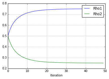
The value of (rho1, rho2) are (0.750, 0.250)
Evaluating the EM algorithm
We will ask two important questions for evaluating whether or not an algorithm is “good.”
Does it converge?
Obviously, we want an algorithm that converges so that the algorithm actually generates estimates. In this case, the algorithm is guaranteed to converge, although it is not guaranteed to converge in general. In general, EM converges if the generative model belongs to the exponential family. More details can be found here.
Is it accurate?
This question is a bit trickier, since we can only evaluate accuracy relative to all other algorithms. We will examine the idea of Maximum Likelihood (ML), a gold standard when assessing algorithms.
Given some reads \(R_1, \dots, R_N\\) for a given model with parameters \(\rho_1, \dots, \rho_k \\), we write the probability of observing the reads \(R_1, \dots, R_N\\) given the parameters \(\rho_1, \dots, \rho_k\\) as \(Pr(R_1, \dots, R_N ; \rho_1, \dots, \rho_k)\). The idea of Maximum Likelihood is that our model should maximize this probability over the parameters. That is, our model should satisfy
\[\max_{\rho_1, \dots, \rho_k} Pr(R_1, \dots, R_N ; \rho_1, \dots, \rho_k).\]As it turns out, the EM algorithm indeed gives the ML result, and thus we can say EM is a good algorithm.