Lecture 17: RNA-seq - De Novo Transcriptome Assembly and Single-Cell RNA-seq
Lecture 17: RNA-seq - De Novo Transcriptome Assembly and Single-Cell RNA-seq
Monday, May 23, 2016
Scribed by the course staff
Topics
De novo transcriptome assembly
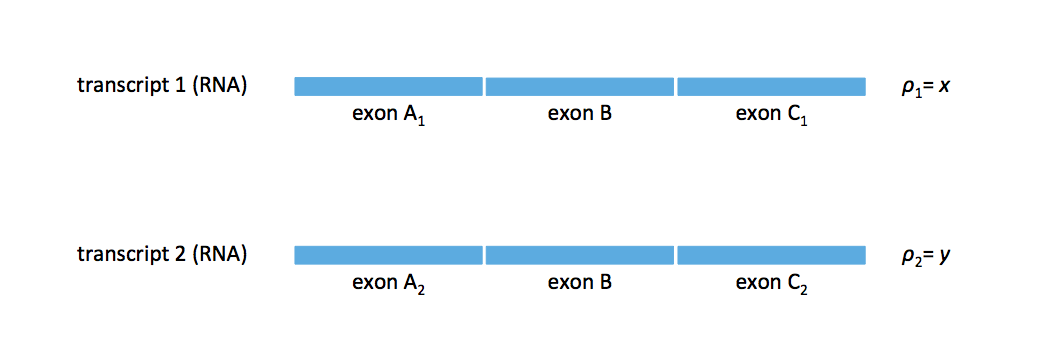
Last time, we ended with the kinds of splicing structures cannot be resolving for the de novo transcriptome assembly problem. We looked at the case where we had two transcripts: \(t_1\) with exons A\(_1\), B, and C\(_1\) and \(t_2\) with exons A\(_2\), B, and C\(_2\) with \(\rho_1 = x\) and \(\rho_2 = y\) with \(x \neq y\). We presented the idea of a splice graph, shown below.
If we assume that two transcripts can resolve this splice graph, we can draw a transcript from A\(_1\) to C\(_1\) and another from A\(_2\) to C\(_2\). When \(x \neq y\), the flows from A\(_1\) to C\(_2\) is ruled out (i.e. the cross-flow solution is ruled out). But we can still have flow patterns with more complex patterns if we relaxed the two-transcript assumption.
Let’s consider what what happen if we assumed 3 transcripts explain this splicing structure. If we assume that \(y > x\), we can start with a flow through \(x\) and then \(y\), resulting in a leftover flow of \(y-x\). We can then draw a flow from \(y\) to \(y\), resulting in a leftover flow of \(x\). Finally, we can draw a third flow from that \(x\) to the remaining \(x\), account for all the abundances. This is summarized in the figure below.
IMAGE OF 3-FLOW GRAPH.
For this example, we assume that each end-to-end flow describes a transcript. With the 3 above flows, we obtain three transcripts with the following abundances: transcript A\(_1\)-B-C\(_2\) with abundance \(x\), transcript A\(_2\)-b-C\(_2\) with abundance \(y-x\), and transcript A\(_2\)-B-C\(_1\) with abundance \(x\). Notice that this solution is not unique, which is not ideal. In a way, however, this solution can already be ruled out because in practice two transcripts are unlikely to have the exact same abundance.
We make the assumption that two transcripts cannot have the same abundance. It’s clear that we need at least 3 transcripts here. We only have 2 degrees of freedom due to the 2 parameters \(x\) and \(y\). In some sense, the 3 numbers associated with the 3 transcripts are constrained in a very specific way. More rigorously, if we think of the abundances of the 3 transcripts as independent random variables, the probability of all 3 abundances lying in a 2-D subspace is essentially 0. This suggests that these repeat problems can be resolved if we assume some sparsity structure.
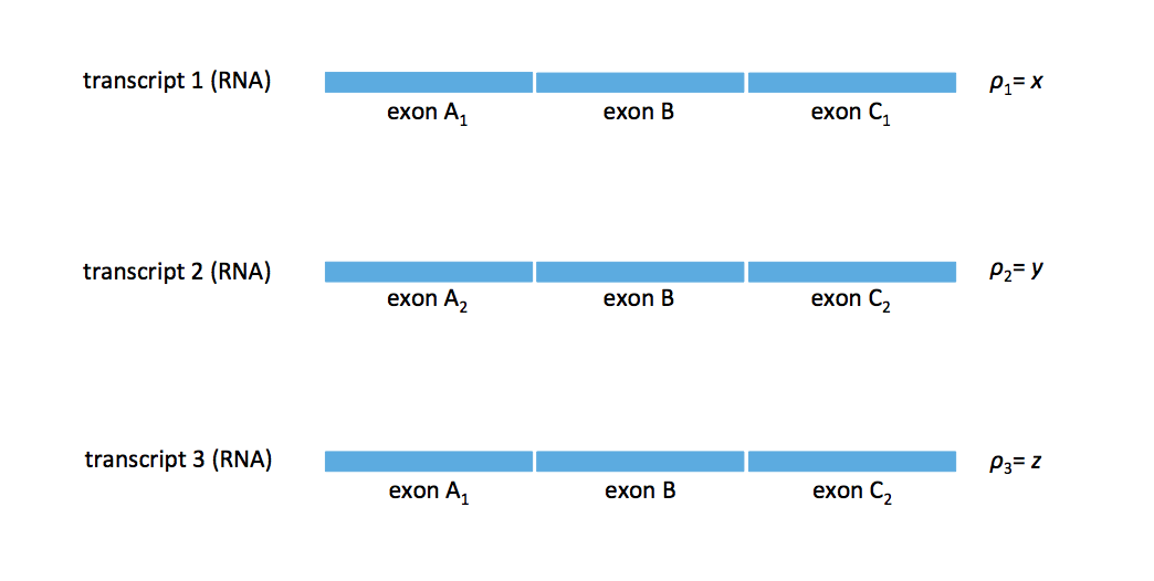
Does there exist a ground truth that results in a splice graph that cannot be resolved unambigiously? Consider the case where we have the 3 transcripts shown in the figure below. In practice, these transcripts can represent 3 isoforms from a particular gene.
The two potential flows that resolve this set of transcript’s splice graph are shown in the figure below.
IMAGE OF THE AMBIGIOUS SPLICE GRAPH
We obtain the alternative solution with \(t_1\) being A\(_1\)-B-C\(_2\), \(t_2\) being A\(_2\)-B-C\(_1\), and A\(_2\)-B-C\(_2\) with \(\rho_1 = x+z\), \(\rho_2 = x\), and \(\rho_3 = y-x\). Furthermore, we cannot rule this alternative solution out. Therefore there does exist certain repeat patterns that we cannot resolve.
A linear-time algorithm for an NP-hard problem
Kannan, Pachter, and Tse implemented an algorithm based on the above sparsest flow concept for their tool Shannon. Specifically, the paper attempts to find the smallest number of end-to-end flows that explain the edge flows based on estimated transcripts. There is still NP-hardness underlying the approach.
If we assume that the abundances are random, then we can eliminate a lot of worse-case sequences that are NP-hard. An example run of the algorithm is shown in the figure below.
IMAGE OF EXAMPLE RUN OF SHANNON’S ALGORITHM
The algorithm attempts to work on the graph locally. Whenever we have some kind of node where we have intersection of flows, we want to tease the flows apart locally first in an attempt to arrive at a global solution. Notice that if we look at only the left-most five nodes, there is some information that we fail to incorporate that could help us. Instead, we can start with the rightmost 4 nodes, resolving the \(a+b\) edge. We now arrive at the only possible sparse set of flows.
Recall that the key object that drives the assembly analysis is \(L_{crit}\). If the read length is less than this, there exist inherent ambiguity to the problem and no algorithm can solve the problem. While the proposed algorithm above can reconstruct in linear time (it doesn’t revisit nodes), it does have a chance of failing due to its greedy nature.
For the mouse transcriptome \(L_{crit} = 4077\), indicating a complex transcriptome structure. While we cannot resolve the transcriptome for all transcripts, we can still recover a significant portion of it. The figure below shows the fraction of transcripts that are reconstructable as a function of read length.
PLOT OF “NEAR-OPTIMALITY AT PRACTICAL L”
This indicates that only a small number of transcripts have complex isoform structures. Automatically when we do sparsest flow, the abundance information is accounted for via the edge weights.
In practice, we have to use the read counts to estimate the abundances. Even if the abundances are generic, if they are close to being non-generic, the estimation error may impose problems. Evaluation on real datasets shows that while Shannon is not perfect, it demonstrates significant improvement over existing tools on some existing datasets.
Single-cell RNA-seq
When sequencing are performed on a piece of tissue (e.g. embryonic stem cells), RNA-seq is performed on many cells at once (bulk sequencing). Therefore the data we obtain are effectively averaged over all these cells. Biologists, however, are also interested in what’s happening on the cell level. Perhaps cells in different stages of development can provide some information for certain phenotypes, for example. How can we invent new methods to do sequencing on a cell-to-cell level?
Single-cell RNA-seq started around 5-7 years ago. Over the years, technologies that could sequence 100s and 1000s of cells emerged.
Drop-seq
More recently, a technology called Drop-seq was introduced; the technology can sequence 10000s of cells. There are few key components to the technology: microfluidics, which separates cells via droplets, and a barcoding scheme, which allows the scientist to obtain more information about each read. Recall that barcoding has also been used in 10X sequencing for detecting which reads come from the same fragment (thus giving us long-range information for applications like phasing).
Drop-seq generates random sequences via “splitting and pooling” for barcodes. Notice we do not need a particular barcode for a particular cell; we just need different barcodes in different cells. By attaching barcode sequences to beads such that different beads get different barcodes, all transcripts attached to the same bead will have the same barcode. After sequencing, we can easily identify which reads come from which cell. A challenge is in ensuring that most droplets have at most one bead.
Drop-seq enables parallel processing of many single-cells at the same time. The first computational problem that one has to solve is in separating reads based on their cell of origin. From each cell, we obtain a vector \(\boldsymbol{\rho}_i \in \mathbb{R}^{20000}\) of abundances of all transcripts within that cell. We will discuss some computational techniques for clustering these high-dimensional vectors next time.